ROUTING ALGORITHM AND KINEMATIC MODEL OF
MOBILE ROBOTS IN WIRELESS SENSORS NETWORKS
Popeanga Catalin
1
and Nicolai Christov
2
1
Departament of Automatic and Industrial Informatic, Politehnica University, Bucharest, Romania
2
Department of System Controlling, Lille 1 University, Lille, France
Keywords: Wireless sensors networks, Routing, Mobile robot, Constraints, Trajectory planning, CFSQP.
Abstract: Mobile wireless sensors networks are a fast changing branch of the wireless networks. The mobility of the
nodes, the trajectory plan and the routing algorithm determine the implementation of a new strategy that
take into account their interdependency with the scope of minimizing the energy consumption and
increasing the coverage grade. The trajectory planning scheme consists of a routing algorithm to maintain
the connectivity and decentralized receding horizon planners that reside on each vehicle to achieve
coordination among agents. The advantage of the proposed algorithm is that each vehicle only requires local
knowledge of its neighboring vehicles.
1 INTRODUCTION
This research concerns the development of mobiles
wireless sensors network based on autonomous
collaborative robots. A node in this network is an
autonomous robot system, self-propelled, with
enough capacity for processing information for
decision-making and sufficient resources to ensure
the implementation of a reduced number of specific
tasks, in an unknown environment (Nicolae and
Dobrescu, 2008).
Many application areas are naturally concerned
by such research. Today, mobile wireless sensors are
becoming increasingly complex, integrate
capabilities of adaptation to various areas of
operation and target ever-increasing demands of
robustness, ergonomics and safety. In addition,
several robots have the opportunity to solve more
efficiently and rapidly a mission.
Most coordinated tasks performed by teams of
mobile wireless nodes, require reliable
communications between the members. Therefore,
task accomplishment requires that nodes navigate
their environment with their collective movement
restricted to coverage area to guarantee integrity of
the communication network.
Maintaining this communication capability
induces physical constraints on trajectories but also
requires calculation of communication variables like
routes and transmitted powers.
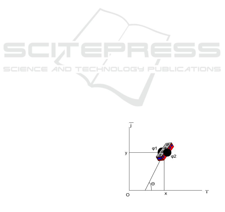
2 ROBOT MODEL
Figure1: The model.
=
cos
=
sin
=
(1)
- The system is subjected to kinematic
constraints (Guo and Parker, 2002), and also to
communication constraints;
459
Catalin P. and Christov N..
ROUTING ALGORITHM AND KINEMATIC MODEL OF MOBILE ROBOTS IN WIRELESS SENSORS NETWORKS.
DOI: 10.5220/0003649604590462
In Proceedings of the 8th International Conference on Informatics in Control, Automation and Robotics (MORAS-2011), pages 459-462
ISBN: 978-989-8425-75-1
Copyright
c
2011 SCITEPRESS (Science and Technology Publications, Lda.)

-The scope of communication is to gather all
information from sensors to a central station, to
have a better coverage and a minimum energy
consume;
-Every node has a start point and a finish point
in the same geographical area.
Decentralized strategies have recently been
introduced. They generally require a
communications flow fairly high in order to transmit
information request to other individuals.
The protocol can include notions of intent and
commitment from which each robot elaborated its
own path, taking into consideration the activities of
other robots.
However, this approach does not fulfill the
constraint on the maintenance communication links.
Other strategies based decentralized fields of
potential (Gazi and Passino, 2004), navigation
functions (potential field without local minimum,
(Gennaro and Jadbabaie, 2006) on the
decomposition cell (Lindhe et al., 2005) have been
developed. However, they are not applicable to the
non-holonomic systems.
Figure 2: Obstacle detection.
Each disc O
mi
is defined by the coordinates of its
center (X
Mi
, Y
mi
) and its radius rmi (1 ≤ mi
d
≤ Mi).
For the avoidance of collisions, the distance
between the robot and obstacles detected Omi time t,
ie
,
()=
(
(
)
−
)
+
(
(
)
−
)
(2)
has to satisfy the inequality :
,
(
)
≥
+
,
∀ ∈
,
,∀
(3)
The planning problem is to compute, in a
cooperative manner, for N robots, allowable
trajectory and collision-free, joining the initial
configuration q
i
(t
initial
), the final configuration
q
i
(T
final
) (with initial velocity u
i
(t
initial
), and final
u
i
(T
final
) assumed to be zero), which optimize the
critter function.
In addition to the individual constraints which
involve only the node itself (ie. constraints non-
holonomy, constraints u
i
ϵ U on the qualifying
speeds and constraints (1) of avoidance robots), the
planned trajectory must respect the constraints
defined here (Desai et al., 1998), (Dunbar and
Murray, 1998), (Defoort et al., 2007d)
.
On the other hand, it is necessary to maintain
some communication links (eg. for an exchange of
strategies for the use of sensors decentralized,
maintain connectedness of training).
To describe the coupling constraints, we can
define the communication graph that will model the
topological structure of the network of com-
communication between vehicles. (Defoort et al.,
2007d).
In general, the performance function is defined
as:
=
(
(
,
,…,
(
)
),
,
,…,
(
)
,)
(4)
where the constraints are:
(
)
,…,
(
)
(
)
=
,
,…,
(
)
=
,
(
)
,…,
(
)
(
)
=
,
,…,
(
)
=
,
(
)
,…,
(
)
(
)
∈
,
(
)
≥
+
,
∀∈
,
,∀
(5)
The trajectory will be projected from q
i
and u
i
in
the flat coordinate z. (Defoort et al., 2007d)
In an unknown environment the planned
trajectory will be available only for a short interval
until the sensors detect obstacles or others robots.
Also for avoiding robots the trajectory planning
can be use, but this approach implies a lot of
communications between nodes. The strategy for
planning the trajectory in such environment is to use
a sliding horizon of time to calculate the new
trajectory. The principle of planning the trajectory is
to divide it in two parts:
- The planning horizon T
p
– represents the interval
for which the performance is evaluated:
- The calculus horizon T
c
– the trajectory is
calculated.
ICINCO 2011 - 8th International Conference on Informatics in Control, Automation and Robotics
460

The critter of performance is then defined as:
=
+
,
−
,
+
(
(
,
)
,
(
,
)
,)
(6)
where L
i
is the cost function and it represents the
energy consumed on every calculated step
to
reach the goal of minimizing the performance
function.
The kinematic of robots influences the messages
passing through the network.
In actual research the topology of the network is
fixed. This introduced a fixed constrain in the
kinematic equation of robots:
(
,
)
≤min
,
,
,
−
(7)
where d
i,com
and d
p.com
are the radio distance covered
by the radio signals at the step
.
The disadvantage of this approach is the
inflexibility of the topology of the network. The
robot sensors cannot cover a large and dynamic area
of interest.
A new approach is needed to have an authentic
influence between the constraints, the energy
consummation, the geographical coverage and the
network coverage.
3 THE ROUTING ALGORITHM
The proposed routing algorithm will use the
information of the planned trajectory of the nodes.
Our network will respect some principles:
The messages will be from the principal node
to the specific node and back,
The main goal of the network is to gather data
from mobile sensors to the principal node,
The role of principal node is to be the network
gateway,
This node will not have kinematic constraints
with respect to the radio links,
The network will be defined in layers, every
layer will represents the number of hops the
message pass from source to destination:
layer (i) - represents the layer on which the
node i is placed in the network, and represents
the number of nodes that a message will pass
from i to node 0.
The new approach will introduce dynamic
constraints. We will consider T
s
as the period these
constraints will be updated.
<
, we will be in the situation of fixed
constraint,
≥
, the routing algorithm will influence the
trajectory planning.
Figure 3: Logical view of the network layers.
At each T
s
, in the network, a SYNC message will
be send in the network with information regarding
the current layer of the transmitter.
And second, there will not be enough time to
calculate the planned trajectory for every possibility
we have to.
Finally the routing algorithm is defined:
The message from node k will be sent to the
node 0 through the node that minimize the
performance critter;
This node is on the next layer close to first
layer;
Every node, from every layer will take the
same decision based on the critter of
performance;
Node 0 will always be on layer 0.
At every interval T
s
the constraints will be
dynamically changed based on the information
broadcasted through the network.
The performance critter will be calculated locally
on each node after the update of the network layers
finish. The second equation (2) becomes:
()
(
,
)
≤min
,
,
(),
−
(8)
where
(
)
∈ ℳ
(
) represents the constraint
node, with it the critter is evaluated and ℳ
(
)
represents the union of the radio linked nodes at
moment:
ℳ
(
)
=
|
≠0,
(
,
)
∈ ℎ
,
(
)
=
(
)
−1 }
(9)
0
2
1
3
4
Layer hop 1
Layer hop 2
ROUTING ALGORITHM AND KINEMATIC MODEL OF MOBILE ROBOTS IN WIRELESS SENSORS NETWORKS
461
4 SIMULATION
For solving the equations we will utilize the function
CFSQP (“Constrained Feasible Sequential Quadratic
Programming”) developed at Maryland University.
This routine utilizes an optimization algorithm based
on sequential quadratic programming
(SQP).(Lawrance et al.,1997)
The SQP is a method iterative where the critter is
changed in an approximated quadratic equation and
the constraints in equations linear. This will permit
to calculate very fast a solution verifying the
constraints.
The robot radius is 0.3 meters and the radio link
is up to 3 meters. The robots will have a maximum
speed of 1 m/s and the orientation will be 0 degree.
In the fixed configuration the existing
approaches are simulated (the network topology will
not influence the planning), in the Fig.2 the new
algorithm is simulated, it will take in consideration
the topology of the network.
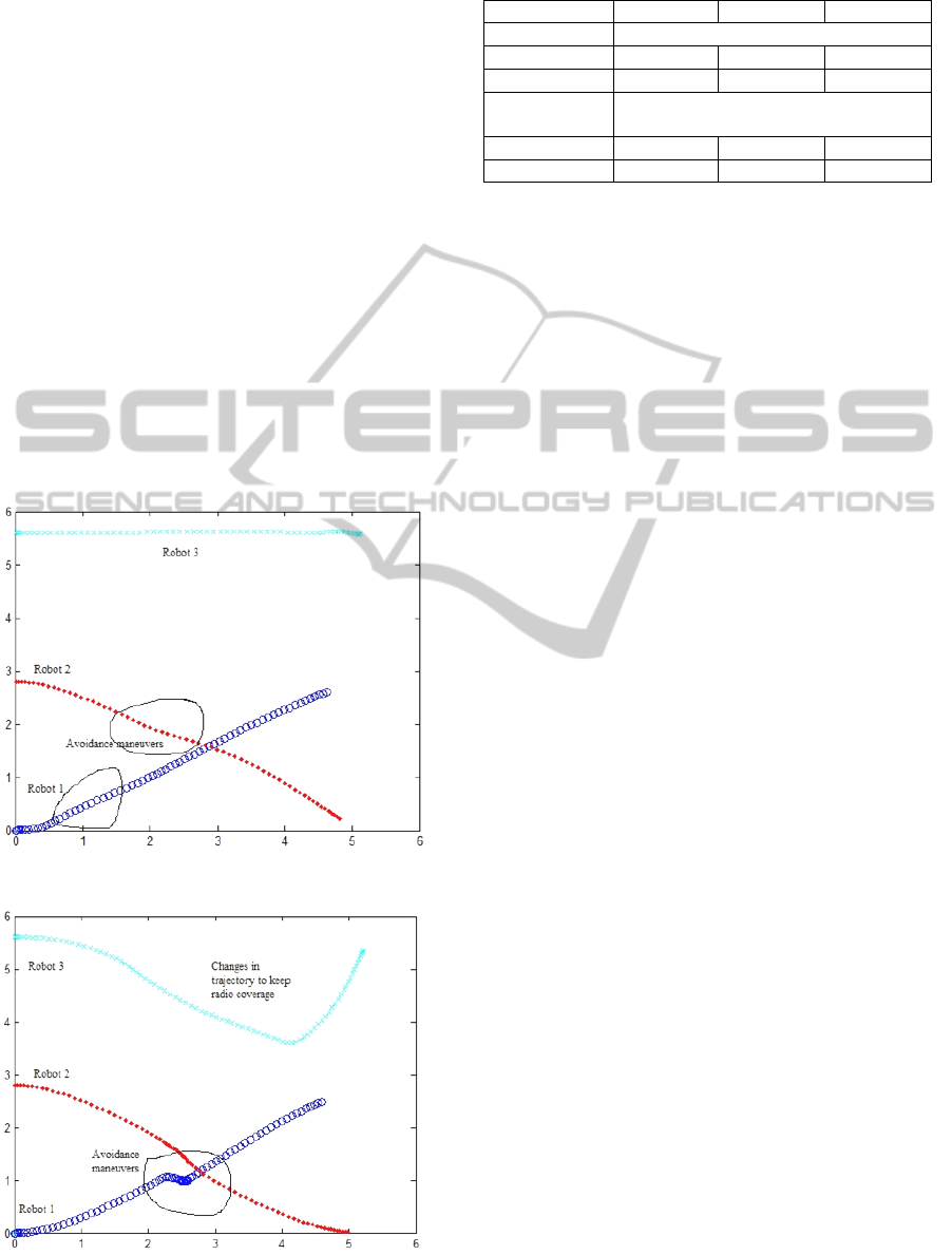
Figure 4: Fixed configuration.
Figure 5: Dynamic configuration.
Table 1: Simulation results.
Nodes 3 6 10
Time (s)
Fix 9.16 9.61 9.77
Dynamic 9.24 12.53 11.92
Radio
Coverage (%)
Fix 70 68 55
Dynamic 100 98 94
5 CONCLUSIONS
In the Table 1, the results of the simulation show the
good potential of this algorithm with dynamic
constraints the radio coverage is substantially
improved from 55-70% of radio communications to
over 94% but with some penalties in the average
time to get to finish.
REFERENCES
Guo, Y. et Parker, L. E. (2002). A distributed and optimal
motion planning approach for multiple mobile robots.
Gazi, V. et Passino, K. (2004). Stability analysis of social
foraging swarms.
Gennaro, M. C. D. et Jadbabaie, A. (2006). Formation
control for acooperative multi-agent system using
decentralized navigation functions.
Lindhe, M., Ogren, P., et Johansson, K. (2005). Flocking
with obstacle avoidance: A new distributed
coordination algorithm based on voronoi partitions.
Michael Defoort (2007), Contribution to trajectory plan
and command of the mobile robots.
Lawrance, C., Zhou, Z., et Tits, A. (1997). User’s guide
for cfsqp version 2.5.Rapport technique, Institute for
Systems Research, University of Maryland.
Defoort, M., Floquet, T., Perruquetti, W., et Boulinguez,
D. (2007d). Experimental motion planning and control
for an autonomous nonholonomic mobilerobot. IEEE
International Conference on Robotics and Automation,
Roma, Italy.
Desai, J., Ostrowski, J., et Kumar, V. (1998). Controlling
formations of multiple mobile robots. IEEE
International Conference on Robotics and Automation,
Leuven, Belgium.
Dunbar, W. et Murray, R. (2002). Model predictive
control of coordinated multi-vehicle formations. IEEE
Conference on Decision and Control.
Nicolae M., Dobrescu R., System for traking, localization
and data acquisition from moving robots through
sensors network, Robotica’08.
ICINCO 2011 - 8th International Conference on Informatics in Control, Automation and Robotics
462
