
INSENSITIVE DIFFERENTIAL EVOLUTION
AND MULTI-SOLUTION PROBLEMS
Itsuki Handa and Toshimichi Saito
Faculty of Science and Engineering, Hosei University, 184-8584 Tokyo, Japan
Keywords:
Swarm inteligence, Differential evolution, Multi-solution problems.
Abstract:
This paper presents an insensitive differential evolution for multi-solution problems. The algorithm consists
of global and local searches. In the global search, the algorithm tries to construct local sub-regions (LSRs)
each of which includes either solution. In the local search, the algorithm operates on all the LSRs in parallel
and tries to find all the approximate solutions. The algorithm has a key parameter that controls the algorithm
insensitivity. If the insensitivity is suitable, the algorithm can construct all the LSRs before trapping into either
solution and can find all the solutions. Performing basic numerical experiments where parameters are adjusted
by trial-and-errors, basic performance of the algorithm is investigated.
1 INTRODUCTION
Differential evolution (DE) is a population-based
search strategy in the evolutionary algorithms (Storn
and Price, 1996) (Storn and Price, 1997) (Storn and
Price, 1995). The DE has particles corresponding
to potential solutions. The particle location is up-
dated by a simple difference equation in order to ap-
proach the optimal solution (Takahama and Sakai,
2004)(Takahama and Sakai, 2006). The DE is sim-
ple, does not require differentiability of the objective
functions and has been applied to various problems
( non-convex, a multi-peak etc.). The engineering
applications are many and include optimal parame-
ter setting of circuits and systems: analog-to-digital
converters (Lampinen and Vainio, 2001), digital fil-
ters (Luitel and Venayagamoorthy, 2008), switching
power converters (Huang et al., 2004), etc.
This paper presents an insensitive differential evo-
lution ( IDE) for multi-solution problems (MSP). The
IDE consists of the global and local searches. In the
global search, the IDE tries to construct local sub-
regions (LSRs) each of which includes either solution.
The IDE has two key parameters: ε controls insensi-
tivity for update of particle position and T
G
controls
switching timing to the local search. As the parameter
ε is small, the algorithm operates similarly to classi-
cal DE where almost all particles tend to converge to
either solution. In such a case, it is hard to maintain a
diversity for successful construction of all the LSRs.
As the parameter ε increases, the algorithm insensitiv-
ity increases and all the LSRs can be constructed be-
fore trapping into either solution. The global search
is stopped at time T
G
and the algorithm is switched
into the local search. In the local search, the IDE op-
erates on all the LSRs in parallel and tries to find all
the approximate solutions. If the global search runs
successfully and can construct all the LSRs, the lo-
cal search can find all the solutions. In the algorithm,
tuning of the two parameters ε and T
G
is very impor-
tant. Performing basic numerical experiments with
trial-and-errors of the parameters tuning, we have in-
vestigated the algorithm performance in several typi-
cal measures such as success rate.
In several evolutionary optimization algorithms
including DEs, escape from a trap of either solution is
a basic issue of the MSPs. The traps relates deeply to
local minima of unique solution problems. In order to
avoid the trap, there exist several strategies including
the tabu search (Li and Zhao, 2010). We believe that
our insensitive method is simpler than existing meth-
ods and can be developed into an effective algorithm
for the MSPs. This paper provides basic information
to develop such an algorithm.
2 INSENSITIVE DIFFERENTIAL
EVOLUTION
We define the algorithm IDE for m-dimensional ob-
jective functions.
292
Handa I. and Saito T..
INSENSITIVE DIFFERENTIAL EVOLUTION AND MULTI-SOLUTION PROBLEMS.
DOI: 10.5220/0003653002920295
In Proceedings of the International Conference on Evolutionary Computation Theory and Applications (ECTA-2011), pages 292-295
ISBN: 978-989-8425-83-6
Copyright
c
2011 SCITEPRESS (Science and Technology Publications, Lda.)

f(~x) ≥ 0, ~x ≡ (x
1
,x
2
,··· ,x
m
) ∈ R
m
(1)
where the minimum value is normalized as 0. This
positive definite function has multiple solutions in the
search space S
0
:
f(~x
i
s
) = 0, i = 1 ∼ N
s
, ~x
i
s
= (x
i
s1
,··· ,x
i
sm
) ∈ S
0
S
0
= {x| |x
1
| ≤ A,··· , |x
m
| ≤ A}
where x
i
s
is the i-th solution (i = 1 ∼ N
s
) and N
s
is the
number of solutions. The search space is normalized
as the center at the original with width A. The IDE has
N pieces of particles whose search is characterized by
the position vectors:
X = {~x
1
,··· ,~x
N
}, ~x
i
≡ (x
i1
,··· ,x
im
) (2)
where i = 1 ∼ N. The vector~x
i
is a potential solution
and is desired to approach either solution. The IDE
consists of two stages. The first stage is the global
search that tries to construct the LSRs each of which
includes either solution. The second stage is the local
search that tries to find the approximate solution in all
the LSRs.
2.1 Global Search
Let t
1
denote the iteration number. The algorithm is
defined by the following 5 steps.
Step 1 (Initialization). Let t
1
= 0. The particles
~x
i
(0) (i = 1 ∼ N) are initialized randomly in S
0
.
Step 2 (Mutation). Three vectors ~x
p1
(t
1
), ~x
p2
(t
1
)
and~x
p3
(t
1
) are selected randomly from the set of par-
ticles X where ~x
p1
(t
1
)6= ~x
p2
(t
1
)6= ~x
p3
(t
1
) is assumed.
A candidate vector~y
i
(t
1
) is made by
~y
i
(t
1
) =~x
p1
(t
1
) + B(~x
p2
(t
1
) −~x
p3
(t
1
)) (3)
where B is the scaling parameter.
Step 3 (Crossover). Applying crossover for the
candidate vector~y
i
≡ (y
i1
,··· ,y
im
) and the parent ~x
i
≡
(x
i1
,··· ,x
im
), we obtain an offspring~c
i
:
(c
i1
,··· ,c
i( j−1)
) = (x
i1
,··· ,x
i( j−1)
)
c
ij
= y
ij
(c
i( j+1)
,··· ,c
im
) =
(y
i( j+1)
,··· ,y
im
) : rate P
c
(x
i( j+1)
,··· ,x
im
) : rate 1− P
c
(4)
where i = 1 ∼ N and P
c
is the crossover probability.
The crossover point j is selected randomly from all
particle subscripts {1, · · · , m}.
Step 4 (Survival). The parent ~x
i
(t
1
) is compared
with the offspring ~c
i
(t
1
) and is updated as the follow-
ing:
~x
i
(t
1
) = ~c
i
(t
1
) if f(~c
i
(t
1
)) < f(~x
i
(t
1
)) − ε
~x
i
(t
1
) =~x
i
(t
1
) if f(~c
i
(t
1
)) > f(~x
i
(t
1
)) − ε
(5)
ε is a key parameter to control the insensitivity.
Step 5. Let t
1
= t
1
+ 1, go to Step 2 and repeat until
the maximum time limit T
G
.
2.2 Local Subregions
The LSRs are constructed based on the set of updated
particles
P = {~x
1
,··· ,~x
N
},
Step 1. Let N
max
denote the upper limit number of
LSRs. Let i be the index of the LSR and let i = 1.
Step 2. The global best particle ~x
g
is selected:
f(~x
g
) ≤ f(~x
i
) for all i
Based on the global best, the i-th LSR is constructed
LSR
i
= { ~x | k~x−~x
g
k< r}
Fig. 1 illustrates the LSR construction. After the
LSR
i
is constructed, all the elements in LSR
i
are re-
moved from P.
Step 3. Let i = i+ 1, go to step 2 and repeat until
the upper limit N
max
.
2.3 Local Search
In the local search, the IDE operates on all the LSRs
in parallel. We define the local search for the LSR
i
.
Let t
2
denotes the iteration number. The particles in
LSR
i
are denoted by
X
i
≡ {~x
1
(t
2
),··· ,~x
N
i
(t
2
)}
The algorithm is defined by the following 5 steps.
×
×
1sol
2sol
×
×
1sol
2sol
1
x
2
x
1
LSR
2
LSR
A
A
A−
A−
Figure 1: Construction of the LSRs.
INSENSITIVE DIFFERENTIAL EVOLUTION AND MULTI-SOLUTION PROBLEMS
293
Step 1 (Initialization). Let t
2
= 0.
Step 2. The mutation is defined by replacing t
1
, X
and N in Step 2 in 2.1 with t
2
, X
i
and N
i
, respectively.
Step 3. The crossover is defined by replacing t
1
, X
and N in Step 3 in 2.1 with t
2
, X
i
and N
i
, respectively.
Step 4 (Survival). The parent ~x
i
(t
2
) is compared
with the offspring ~c
i
(t
2
) and is updated as the follow-
ing:
~x
i
(t
2
) = ~c
i
(t
2
) if f(~c
i
(t
2
)) < f(~x
i
(t
2
)) − ε
2
~x
i
(t
2
) =~x
i
(t
2
) if f(~c
i
(t
2
)) > f(~x
i
(t
2
)) − ε
2
(6)
ε
2
is a key parameter to control the insensitivity in the
local search. Let f(~x
Li
) is the best in the LSR
i
. The
algorithm is terminated if
f(~x
Li
) ≤ C
1
where C
1
is an approximation criterion and~x
Li
is the
approximate solution. Otherwise, go to Step 5.
Step 5: Let t
2
= t
2
+ 1, go to Step 2 and repeat until
the maximum time limit T
L
.
3 NUMERICAL EXPERIMENTS
In order to confirm the algorithm efficiency, we have
performed basic numerical experiments for a two di-
mensional function.
f
1
(~x) = −0.397+ (x
2
−
5.1
4π
2
1
x
2
1
+
5
π
x
1
− 6)
2
+(1−
1
8π
)cos(x
1
) + 10
S
0
= {(x
1
,x
2
)| |x
1
| ≤ 15, |x
2
| ≤ 15 }
(7)
f
1
has three solutions as illustrated in Fig. 2(a):
min( f
1
(~x)) = 0
~x
1
s
.
= (−π, 12.3), ~x
2
s
.
= (π,2.28), ~x
3
s
.
= (9.42, 2.48)
We have selected insensitive parameters (ε, ε
2
) and
the global search time limit T
G
as control parame-
ters. Other parameters are fixed after trial-and-errors:
the number of particle N=30, the scaling parameter
B=0.7, crossover probability P
c
=0.9, approximation
criterion C
1
= 0.01, the upper limit number of LSRs
N
max
=3, LSR radius r=1 and the maximum time step
of the local search T
L
=70.
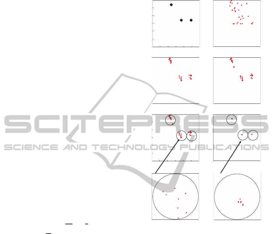
Fig. 2 (b)-(d) show particle movement in global
search for ε=3.0 and T
G
=30. At t = T
G
= 30, the par-
ticles are divided into three swarms and the global
search is stopped. The algorithm constructs three
LSRs as shown in Fig. 2 (e) where each LSR in-
cludes either solution. The algorithm is switched into
0)b(
1
=t
15
15)c(
1
=t
30)d(
1
=t
1
s
x
r
)a(
15
0
0
15−
15−
1
x
2
x
)50(20)f(
12
== tt
)30(0)e(
12
== tt @
×
×
×
× ×
)e(
'
)f(
'
15
15
0
0
15−
15−
2
x
1
x
2
s
x
r
3
s
x
r
Figure 2: Particles movement for ε=3.0, T
G
=30, ε
2
=0.01
and T
L
=70. (a) Solutions, (b) to (d) global search, (d) to (f’)
local search.
the local search with ε
2
= 0.01 and can find all the ap-
proximatesolutions within the time limitt
2
= T
L
= 70.
Fig. 2 (f) shows that particles in each LSR converge
to the each approximate solution. Figs. 2 (e’) and (f’)
show enlargement of LSR
2
in Figs. 2 (e) and (f), re-
spectively. Fig. 3 shows the local search process for
ε
2
=0.01 and T
L
=70. The global search is said to be
successful if the IDE can construct all the LSRs in-
cluding either solution and local search is said to be
successful if all the solutions are found.
Table 1 shows the success rate (SR) of global
search for different initial particles positions, muta-
tion and crossover in 50 trials. We can see that a good
SR can be realized around (ε,T
G
) = (3,30). The in-
sensitive parameter ε plays an important role to con-
struct the LSRs. If the parameter ε is too small then
the IDE operation is the almost same as the standard
DE and all the particles tend to be attracted to one so-
ECTA 2011 - International Conference on Evolutionary Computation Theory and Applications
294

Table 1: Success rate (SR) of global search.
H
H
H
H
T
G
ε
0 1 2 3 4 5
10 36 72 80 80 72 68
20 36 68 68 84 84 72
30 44 74 84 88 80 76
40 26 64 70 80 88 82
50 4 68 72 78 76 80
Table 2: SR of local search for successful global search
(ε=3, T
G
= 30).
ε
2
0.01 0.02 0.1 0.5 1.0 2.0 3.0
SR 100 100 60 10 1 0 0
1.E-03
1.E-02
1.E-01
1.E+00
1.E+01
1.E+02
30 40 50
Criterion
1op
2op
3op
2
t
)( xF
r
Figure 3: Local search process for ε
2
=0.01 and T
L
=70.
0)a(
1
=t
30)b(
1
=t
15
15
0
0
15−
15−
2
x
1
x
Figure 4: Particles movement of global search for ε=0.
50)b(
1
=t
30)a(
1
=t
15
15
0
0
15−
15−
1
x
2
x
Figure 5: Particles movement (t
1
≥ 30) if the global search
continues after Fig. 2 (d).
lution as suggested in Fig. 4 for ε = 0. In this case,
the IDE can not find all the three solutions. If ε is too
large then to IDE is too insensitive to find LSRs. The
global search limit T
G
is also important. If the global
search continues after the time limit T
G
then particles
in either swarm tend to be attracted to other swarms
as suggested in Fig. 5. If ε is too small or T
G
is too
large, the particles converge to one solution. Table 2
shows the SR of local search for 50 trials where ε=3,
T
G
=30 and the SR is calculated for successful global
search. The SR=100 is achieved for small ε and the
SR decreases as ε
2
increases.
4 CONCLUSIONS
A basic version of the IDE is presented and its per-
formance is investigated in this paper. In the global
search, the IDE can construct the LSRs successfully
if the key parameters ε and T
G
are selected suitably.
In the local search, the IDE can find the desired ap-
proximate solution almost completely if ε
2
is selected
suitably.
Future problems are many, including analysis of
search process, analysis of insensitive parameters ef-
fects, automatic adjustment of key parameters, appli-
cation to various functions, comparison with existing
algorithms and application to engineering problems.
REFERENCES
Huang, H., Hu, S., and Czarowski, D. (2004). Harmonic
elimination for constrained optimal pwm. In Proc.
Annual Conf. IEEE Ind. Electron. Soc., pages 2702–
2705.
Lampinen, H. and Vainio, O. (2001). An optimization ap-
proach to designing otas for low-voltage sigma-delta
modulators. In Proc. of WCCI, pages 1665–1671.
Li, C. and Zhao (2010). The hybrid differential evolution
algorithm for optimal power flow based on simulated
annealing and tabu search. In Proc. of IEEE, pages
1–7.
Luitel, B. and Venayagamoorthy, G. (2008). Differential
evolution particle swarm optimization for digital filter
design. In Proc. of IEEE, pages 3954–3961.
Storn, R. and Price, K. (1995). Differrential evolution - a
simple and efficient adaptive scheme for global opti-
mization over continuous spaces. In ICSI Technical
Report, International Computer Science Institute.
Storn, R. and Price, K. (1996). Minimizing the real func-
tions of the icec’96 contest by differential evolution.
In Proc. of ICEC, pages 842–844.
Storn, R. and Price, K. (1997). Differrential evolution - a
simple and efficient heuristic for global optimization
over continuous spaces. In Journal of Global Opti-
mization, pages 341–359.
Takahama, T. and Sakai, S. (2004). Constrained optimiza-
tion by combining the α constrained method with par-
ticle swarm optimization. In Proc. of Joint 2nd In-
ternational Conference on Soft Computer and Intelli-
gent Systems and 5th International Symposium on Ad-
vanced Intelligenct Systems.
Takahama, T. and Sakai, S. (2006). Constrained opti-
mization by the ε constrained differential evolution
withgradient-based mutation and feasible elites. In
Proc. of WCCI, pages 308–315.
INSENSITIVE DIFFERENTIAL EVOLUTION AND MULTI-SOLUTION PROBLEMS
295
