
ENSEMBLE RANDOM-SUBSET SVM
Kenji Nishida, Jun Fujiki
Human Technology Research Institute, National Institute of Advanced Industrial Science and Technology (AIST)
Central 2, 1-1-1 Umezono, Tsukuba-shi, 305-8568 Ibaraki, Japan
Takio Kurita
Faculty of Engineering, Hiroshima University, 1-4-1 Kagamiyama, Higashi-Hiroshima-shi, 739-8527 Hiroshima, Japan
Keywords:
Ensemble learning, Bagging, Boosting, Generalization performance, Support vector machine.
Abstract:
In this paper, the Ensemble Random-Subset SVM algorithm is proposed. In a random-subset SVM, multi-
ple SVMs are used, and each SVM is considered a weak classifier; a subset of training samples is randomly
selected for each weak classifier with randomly set parameters, and the SVMs with optimal weights are com-
bined for classification. A linear SVM is adopted to determine the optimal kernel weights; therefore, an
ensemble random-subset SVM is based on a hierarchical SVM model. An ensemble random-subset SVM out-
performs a single SVM even when using a small number of samples (10 or 100 samples out of 20,000 training
samples for each weak classifier); in contrast, a single SVM requires more than 4,000 support vectors.
1 INTRODUCTION
Although support vector machines (SVMs)(Vapnik,
1998; Sch¨olkopf et al., 1999; Cristiani and Tay-
lor, 2000) provide high accuracy and generalization
performance, large amount of computation time and
memory are required when they are applied to large-
scale problems. Therefore, many previous works at-
tempted to resolve these problems. For example,
Chapelle examined the effect of optimization of SVM
algorithm (Chapelle, 2007), which reduces the com-
putation complexity from O(n
3
) (for naive imple-
mentation) to about O(n
2
sv
) (n
sv
denotes the num-
ber of support vectors), and Keerthi proposed to re-
duce the number of kernels with forward stepwise se-
lection and attained a computational complexity of
O(nd
2
) (Keerthi at al., 2007), where d denotes the
number of selected kernels. Lin proposed to se-
lect a random subset of the training set (Lin and
Lin, 2003); however, this approach could not re-
duce the number of basis functions to attain an ac-
curacy close to that of a full SVM solution. Demir
applied the RANSAC(Fischler et al.,1981) algorithm
to reduce the number of training samples for the
Relevance-VectorMachine (RVM) for remote sensing
data (Demir, 2007). Nishida proposed the RANSAC-
SVM (Nishida and Kurita, 2008) to reduce the num-
ber of training samples for improving generalization
performance. In the RANSAC-SVM, an SVM is
trained using a randomly selected subset of training
samples, and hyper-parameters (such as a regulariza-
tion term and Gaussian width) are set to fit over whole
training samples. Though RANSAC-SVM effectively
reduced the computation time required for training by
reducing the number of training samples, a large num-
ber of trials were required to determine a combina-
tion of good subset samples and good hyperparame-
ters (e.g., 100,000 trials were performed in (Nishida
and Kurita, 2008)). The hyperparameters for a single
SVM must be strictly determined to simultaneously
achieve high classification accuracy and good gen-
eralization performance. Therefore, RANSAC-SVM
had to perform an exhaustive search for good param-
eters.
Many ensemble learning algorithms have been
proposed for improving the generalization perfor-
mance such as boosting (Freund and Schapire, 1996)
and bagging (Breiman, 1998). In ensemble learning,
the weak classifiers must maintain high generaliza-
tion performance, but high classification accuracy is
not required for each weak classifier because an accu-
rate classification boundary is determined by combin-
ing the weak (low classification accuracy) classifiers.
Therefore, we have an opportunity of avoiding an ex-
334
Nishida K., Fujiki J. and Kurita T..
ENSEMBLE RANDOM-SUBSET SVM.
DOI: 10.5220/0003668903340339
In Proceedings of the International Conference on Neural Computation Theory and Applications (NCTA-2011), pages 334-339
ISBN: 978-989-8425-84-3
Copyright
c
2011 SCITEPRESS (Science and Technology Publications, Lda.)

haustive search for the appropriate hyperparameters,
by providing a variety of weak classifiers. In this pa-
per, we propose the Ensemble Random-Subset SVM,
which is a natural extension of the RANSAC-SVM,
for ensemble learning.
The rest of the paper is organized as follows. In
Section 2, we describe the Ensemble Random-Subset
SVM algorithm. In Section 3, we present the ex-
perimental results for an artificial dataset. Ensem-
ble Random-Subset SVM showed good classification
performance and outperformed a single SVM for the
same test samples.
2 ENSEMBLE RANDOM-SUBSET
SVM
The algorithm of an ensemble random-subset SVM is
presented in this section. We first introduce the pre-
vious works on learning algorithms that use subsets
of training samples, and then, we introduce the defi-
nition of an ensemble kernel SVM, that uses subsets
of training samples.
2.1 Learning Algorithms using Subsets
of Training Samples
Several algorithms that use a subset of training sam-
ples havebeen proposed previously. These algorithms
can be used to improve the generalization perfor-
mance of classifiers or to reduce the computation cost
for the training. Feature vector selection (FVS) (Bau-
dat, 2003) has been used to approximate the feature
space F spanned by training samples by the subspace
F
s
spanned by selected feature vectors (FVs). The
import vector machine (IVM)(Zhu and Hastie, 2005)
is built on the basis of kernel logistic regression and
is used to approximate the kernel feature space by
a smaller number of import vectors (IVs). Whereas
FVS and IVM involve the approximation of the fea-
ture space by their selected samples, RANSAC-SVM
(Nishida and Kurita, 2008) involves the approxima-
tion of the classification boundary by randomly se-
lected samples with optimal hyperparameters. In the
cases of FVS and IVM, the samples are selected se-
quentially, but in the case of RANSAC-SVM, samples
are selected randomly; nevertheless, in all these cases,
a single kernel function is used over all the samples.
SABI (Oosugi and Uehara, 1998) sequentially se-
lected a pair of samples at a time and carried out linear
interpolation between the samples in the pair in or-
der to determine a classification boundary. Although
SABI does not use the kernel method, the combina-
tion of classification boundaries in SABI can be con-
sidered as a combination of different kernels.
An exhaustive search for the optimal sample sub-
set requires a large amount of computation time;
therefore, we employed random sampling to select
subsets and combined multiple kernels with differ-
ent hyper-parameters for the subsets for ensemble
random-subset SVM.
2.2 Ensemble Kernel SVM
The classification function is given as
f(x) = sign(w
T
φ(x) − h). (1)
where function sign(u) is a sign function, which
outputs 1 when u > 0 and outputs -1 when u ≤ 0;
w denotes a weight vector of the input; and h denotes
a threshold. φ(x) denotes a nonlinear projection of
an input vector, such as φ(x
1
)
T
φ(x
2
) = K(x
1
, x
2
). K
is called a Kernel Function and is usually a simple
function, such as the Gaussian function
K(x
1
, x
2
) = exp
−||x
1
− x
2
||
2
G
. (2)
Substituting equation (2) in equation (1), we ob-
tain the following classification function:
f(x) = sign(
∑
i
α
i
t
i
K(x
i
, x) − h), (3)
where α
i
denotes the sample coefficients.
On the basis of equation (3), the classification
function for ensemble kernel SVM is determined as
follows:
f(x) =
p
∑
m=1
β
m
n
∑
i=1
α
m
i
t
i
K(x
i
, x) − h, (4)
where n is the number of sample; α
m
i
, the weight
coefficient; and t
i
, the sample label. The kernel
weights satisfy the conditions β
m
≥ 0 and
∑
p
m=1
β
m
=
1. Different kernels (such as linear, polynomial, and
Gaussian kernels) or kernels with different hyper-
parameters (for example, Gaussian kernels with dif-
ferent Gaussian widths) can be combined; however,
the same weight is assigned to a kernel over all the
input samples, as per the definition in equation (4).
In the ensemble SVM described in equation (4),
all the training samples are used to determine a ker-
nel matrix. However, kernels over different subsets of
training samples can be combined; for example,
f(x) =
p
∑
m=1
β
m
∑
i∈
˙
X
α
m
i
t
i
hK
m
(x, x
i
)i + h, (5)
where
˙
X denotes the subset of training samples for
the m-th kernel, and X denotes the full set of training
ENSEMBLE RANDOM-SUBSET SVM
335
samples. The sampling policy for the subsets is not
restricted to any method, but if the subsets are sam-
pled according to the probability distribution η
m
(x),
the kernel matrix is defined as follows:
K
η
(˙x
i
, ˙x
j
) =
p
∑
m=1
hΦ
m
(˙x
i
), Φ
m
( ˙x
j
)i, (6)
where
˙
X = ηX. The probability that K
η
(˙x
i
, ˙x
j
) is ob-
tained becomes the product of the probabilities of ob-
taining x
i
and x
j
.
2.3 Subset Sampling and Training
Procedure
Because the subset kernel (K
m
) is determined by the
subset of training samples (
˙
X
m
), the subset selection
strategy may affect the classification performance of
each kernel. Therefore, in a random-subset SVM, the
following three parameters must be optimized: sam-
ple weight α
m
i
, kernel weight β
m
, and sample sub-
set
˙
X
m
. However, since simultaneous optimization of
three parameters is a very complicated process, we
generate randomly selected subsets to determine α
m
i
s
for a subset kernel with randomly assigned hyper-
parameters; then, we determine β
m
as the optimal
weight for each kernel. When the kernel weights β
m
are maintained to be optimal, the weights for kernels
with insufficient performancebecome low. Therefore,
such kernels may not affect the overall performance.
A RBF SVM is employed for each weak classifier
f
m
(x), and an ensemble random-subset SVM is im-
plemented in the form of a hierarchical SVM. There-
fore, we first optimize the sample weights α
i
for each
subset-kernel SVM f
m
(x) and then optimize the clas-
sifier weights β
m
. We employed the additive approach
for determining a new weak classifier to maintain the
generalization performance for the integrated classi-
fier. The detailed algorithm is as follows:
1. Let n be the number of training samples X; M,
be the number of kernels; Q, be the number of
samples in the selected subsets
˙
X
m
; and R, be the
number of trials for the parameter selection.
2. Repeat the following steps M times ({m =
1. . . M}):
(a) Repeat the following steps R times ({r =
1. . . R}):
i. Determine a training subset
˙
X
r
m
by randomly
selecting Q samples from X .
ii. Randomly set hyperparameters (such as the
Gaussian width and the regularization term for
the RBF kernel).
iii. Train the m-th classifier f
r
m
over the subset
˙
X
r
m
.
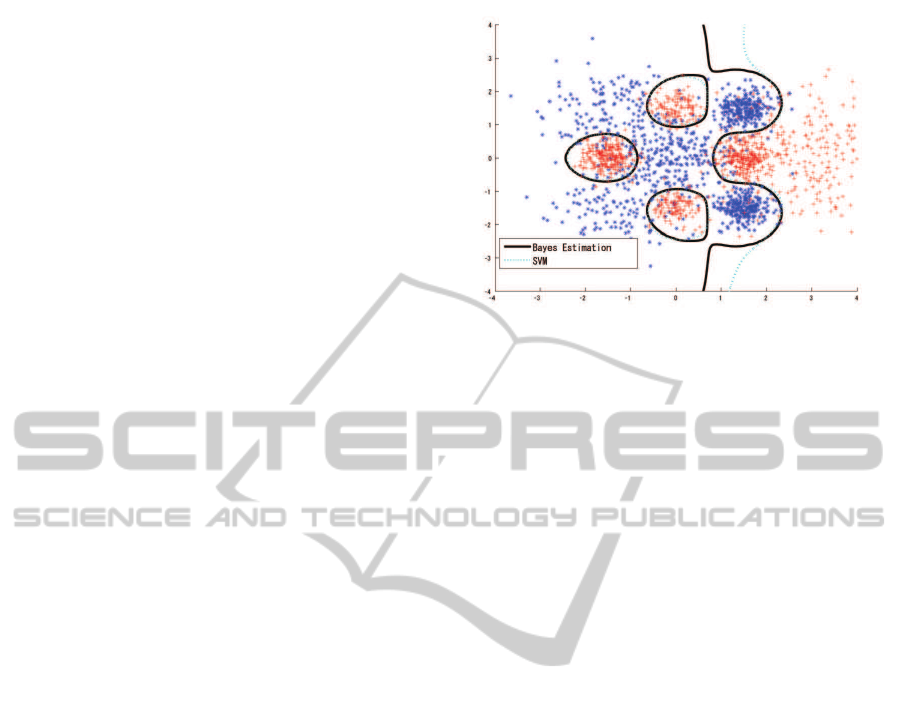
Figure 1: Experimental Data and Classification Boundary.
Black line indicates classification boundary for Bayesian
estimation. Blue dashed line indicates classification bound-
ary for a single SVM.
iv. Predict all training samples X using f
r
m
, to de-
termine the probability output.
v. Train a linear SVM over { f
1
. . . f
m−1
, f
r
m
} to
determine the optimal β
r
m
in order to obtain
the temporal integrated classifier F
r
m
.
(b) Select the f
r
m
that gives the optimal F
r
m
to be the
m-th weak classifier f
m
.
3. Train a linear SVM over f
1
. . . f
M
to determine the
optimal β
M
in order to obtain the final classifier
F
M
.
3 EXPERIMENTAL RESULTS
The experimental results are discussed in this section.
Although a wide variety of kernels are suited for use
in ensemble random-subset SVM, we use only RBF-
SVM for the subset SVMs to investigate the effect
of random sampling. Hyperparameters (G and C for
LIBSVM (Chang and Lin, 2001)) are randomly set to
the desired range for the dataset. We employed linear
SVM to combine the subset kernels in order to obtain
the optimal kernel weight for classification.
3.1 Experimental Data
We evaluated the ensemble random-subset SVM by
using the artificial data in this experiment. The data
are generated from a mixture of ten Gaussian distribu-
tions; of these, five generate class 1 samples, and the
other five generate class –1 samples. 10,000 samples
are generated for each class as training data, and an-
other 10,000 samples are independently generated for
each class as test data. The contour in figure 1 indi-
cates the Bayesian estimation of the class boundary;
NCTA 2011 - International Conference on Neural Computation Theory and Applications
336
the classification ratio for the Bayesian estimation is
92.25% for the training set and 92.15%for the test set.
The classification ratio for the full SVM, in which the
parameters are determined by five-fold cross valida-
tion (c = 3 and g = 0.5), is 92.22% for the training
set and 91.95% for the test set (figure 1), with 4,257
support vectors.
The fitting performance of a random-subset SVM
may be affected by the size of the subset; therefore,
we evaluated a small subset (10-sample subset) and
a larger subset (100-sample subset). All the experi-
ments were run three times, and the results were aver-
aged.
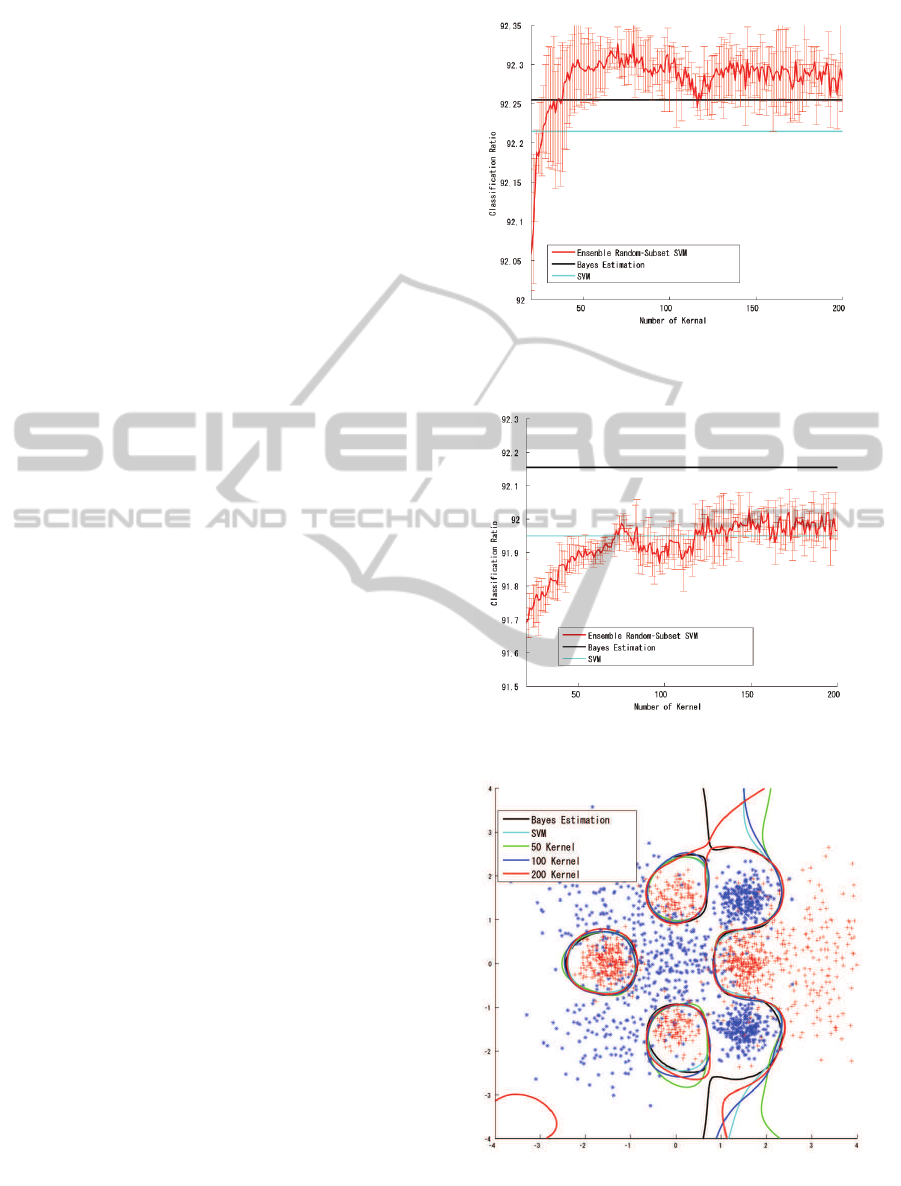
3.2 10-sample Subset SVM
We first examined the 10-sample subset SVM. Five
sets of parameters (C and G) were generated ran-
domly and evaluated for a 10-sample subset. Then,
the parameter set that yielded the best classification
ratio for all training samples was selected for the sub-
set SVM. We generated five sample subset candidates
at a time and thus evaluated 25 subset/parameter sets
in the selection procedure.
Figure 2 shows the classification ratio for the
training samples, and figure 3 shows the classifica-
tion ratio for the test samples. The classification ratio
for the training samples converged quickly, exceed-
ing the Bayesian estimation for 40 kernels and finally
reached 92.26% for 200 kernels. Although this in-
dicated slight over-fitting for the training samples, the
classification ratio for the test samples indicated fairly
good classification performance (comparable with the
result of the full SVM) and reached 91.98% for 200
kernels.
The classification boundary in figure 4 also in-
dicates stable classification performance for the 10-
sample subset.
3.2.1 100-sample Subset SVM
Figures 5 and 6 show the classification ratio for the
100-sample subset SVM with parameter selection for
the training samples and the test samples respectively.
The result showed a trend similar to that observed
for the 10-sample subset-SVM; slight over-fitting was
observed for the training samples (92.26% for 200
kernels), and the classification ratio was similar to the
SVM result for the test samples (91.98% at 200 ker-
nels). As figure 7 shows, the classification boundary
obtained by the 100-sample subset SVM is very sim-
ilar to that obtained by the Bayesian estimation.
Figure 2: Result for 10-Sample Subset SVM (Training).
Figure 3: Result for 10-Sample Subset SVM (Test).
Figure 4: Classification Boundary for 10-Sample Subset
SVM.
ENSEMBLE RANDOM-SUBSET SVM
337
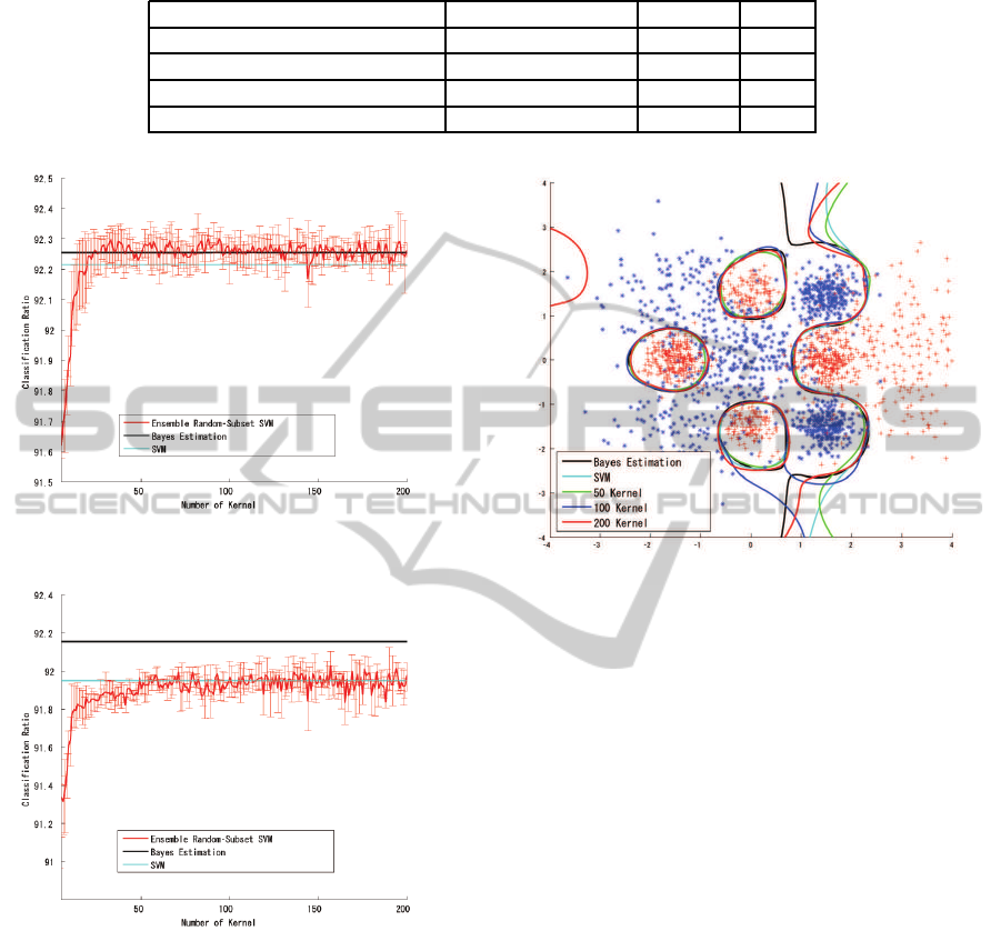
Table 1: Classification Ratio for
cod-rna
dataset.
Number of kernels Training Test
Single SVM (Full set) 1 95.12 96.23
Ensemble SVM subset = 500 3000 95,03 96.16
Ensemble SVM subset = 1000 2000 95.30 96.30
Ensemble SVM subset = 5000 100 94.90 96.24
Figure 5: Result for 100-Sample Subset SVM (Training).
Figure 6: Result for 100-Sample Subset SVM (Test).
3.3 Result for Benchmark Set
Next, we examined a benchmark set
cod-rna
from
the LIBSVM dataset (Libsvm-Dataset). The
cod-rna
dataset has eight attributes, 59,535 training samples,
and 271,617 validation samples with two-class labels.
Hyperparameters for a single SVM were obtained by
performing a grid search through five-fold cross val-
idation, whereas the hyperparameters for the ensem-
ble random-subset SVM were set such that their val-
ues were close to the values for the single SVM. We
applied the random-subset SVM for this dataset be-
cause the dataset includes a large number of samples.
Figure 7: Classification Boundary for 100-Sample Subset
SVM.
We examined 500-sample, 1000-sample, and 5000-
sample subsets.
Table 1 shows the results for the
cod-rna
dataset.
The ensemble random-subset SVM outperformed the
single SVM with a subset size of 1,000 (1.7% of
the total number of the training samples) combining
2,000 SVMs and with a subset of 5,000 (8.3% of the
training samples) combining 100 SVMs.
4 CONCLUSIONS
We proposed an ensemble random-subset SVM algo-
rithm, which combines multiple kernel SVMs gener-
ated from small subsets of training samples.
The 10-sample subset-SVM outperformed the sin-
gle SVM (4,257 support vectors), combining about
120 subset SVMs, and the 100-sample subset SVM
also outperformed the single SVM, combining about
50 subset-SVMs. The use of a larger subset (100-
sample subset) not only helped accelerate the conver-
gence of the classifier but also slightly improved the
final classification ratio.
The result for the benchmark dataset
cod-rna
showed that an ensemble random-subset SVM with
a subset size of 2% or 5% of the training samples can
NCTA 2011 - International Conference on Neural Computation Theory and Applications
338

outperform a single SVM with optimal hyperparame-
ters.
Although 200 or 2000 SVMs must be combined
in an ensemble random-subset SVM, the number of
computations for the subset-kernels would not exceed
that for a single (full-set) SVM because an SVM re-
quires at least O(N
2
) to O(N
3
) computations.
We employed a linear SVM to combine the ker-
nels and obtained the optimal kernel weights. How-
ever, this final SVM took up the majority of the com-
putation time of the ensemble random-subset SVM
because it had to be trained for as many samples as
the large-attribute training samples.
In this study, we used all the outputs from subset
kernels for the training samples; however, we can ap-
ply feature selection and sample selection for the final
linear SVM, as this may help reduce the computation
time and improve the generalization performance si-
multaneously.
REFERENCES
Baudat, G. “Feature Vector Selection and Projection Using
Kernels”, in NeuroComputing, Vol.55, No.1, pp.21-
38, 2003.
Breiman, L. “Bagging Predictors”, Machine Learning,
Vol.24, pp.123-140, 1996.
Chang, C. C. and Lin, C. J. “LIBSVM: a
library for support vector machines”,
http://www.csie.ntu.edu.tw/˜cjlin/libsvm, 2001.
Chapelle, O. “Training a Support Vector Machine in the Pri-
mal”, in Large-Scale Kernel Machines, pp.29-50, The
MIT Press, 2007.
Cristianini, N. and Taylor, J. S. An Introduction to Sup-
port Vector Machines and other kernel-based learning
methods, Cambridge University Press, 2000.
Demir, B. and Erturk, S. “Hyperspectral Image Classifica-
tion Using Relevance Vector Machines”, IEEE Geo-
science and Remote Sensing Letters, Vol.4, No.4,
pp.586-590, 2007.
Fischler, M. A. and Bolles, R. C. “Random Sample Con-
sensus: A Paradigm for Model Fitting with Appli-
cations to Image Analysis and Automated Cartogra-
phy”, Communications of the ACM, Vol.24, pp.381-
395, 1981.
Freund, Y. and Schapire, R. E. “Experiments with a New
Boosting Algorithm”,in Proc. of International Conf.
on Machine Learning (ICML96), pp.148-156, 1996.
Keerthi, S. S. and Chapelle, O. and DeCoste, D. “Build-
ing SVMs with Reduced Classifier Complexity”, in
Large-Scale Kernel Machines, pp.251-274, The MIT
Press, 2007.
Lin, K.-M. and Lin, C.-J. “A Study on Reduced Support
Vector Machines”, IEEE Transactions on Neural Net-
works, Vol.14, pp.1449-1459, 2003.
Nishida, K. and Kurita, T. “RANSAC-SVM for Large-Scale
Datasets”, in proc. International COnference on Pat-
tern Recognition (ICPR2008), 2008. (CD-ROM).
Oosugi, Y. and Uehara, K. “Constructing a Minimal
Instance-base by Storing Prototype Instances”, in J.
of Information Processing, Vol.39, No.11, pp.2949-
2959, 1998. (in Japanese).
Sch¨olkopf, B. and Burges, C. J. C. and Smola, A. J. Ad-
vances in Kernel Methods - Support Vector Learning,
The MIT Press, 1999.
Vapnik, V. N. Statistical Learning Theory, John Wiley &
Sons, 1998.
Zhu, J. and Hastie, T. “Kernel Logistic Regression and
the Import Vector Machine”, J.of Computational and
Graphical Statistics, Vol.14, No.1, pp.185-205, 2005.
LIBSVM data set, http://www.csie.ntu.edu.tw/˜cjlin/libsvm
tools/datasets/binary.html#cod-rna, 2006.
ENSEMBLE RANDOM-SUBSET SVM
339
