
HAMILTONIAN NEURAL NETWORK-BASED ORTHOGONAL
FILTERS
A Basis for Artificial Intelligence
Wieslaw Citko and Wieslaw Sienko
Department of Electrical Engineering, Gdynia Maritime University, Morska 81-86, 81-225, Gdynia, Poland
Keywords: Hamiltonian neural network, Machine learning, Artificial intelligence.
Abstract: The purpose of the paper is to present how very large scale networks for learning can be designed by using
Hamiltonian Neural Network-based orthogonal filters and in particular by using octonionic modules. We
claim here that octonionic modules are basic building blocks to implement AI compatible processors.
1 INTRODUCTION
It is well known that true artificial intelligence
cannot be implemented with traditional hardware.
However, it should also be clear that in order to
build machines that learn, reason and recognize one
needs power-efficient processors with computational
efficiency unattainable even by supercomputers.
Two such processors are theoretically known:
quantum computers and neuromophic or brain-like
structures. Unfortunately, in recent years, quantum
computers have lost much of their luster. Some
researchers are sceptical about eventual realization
of quantum computers (Gea-Banacloche, 2010). One
of the Nobel Prize winners even claims that the ideal
quantum computer can never be built: “no quantum
computer can ever be built that can outperform a
classical computer if the latter would have its
components and processing speed scaled to Planck
units” (Hooft, 2000). The main premise for the claim
above is the essential and unavoidable decoherence
in quantum systems. Thus, due to the decoherence,
an ideal quantum computer as the state superposition
based processor cannot be constructed. It is also
worth noting that an ideal quantum computer is an
example of a Hamiltonian system. As mentioned
above the other way leading to the realization of
power-efficient processors involves neuromorphic
systems. It is well known that up to date, using
different technology, several neuromorphic devices
(e.g. oscillatory and static artificial neurons and
based on them structures) have been proposed (Basu
and Hasler, 2010). The newest project in this field is
memristor concept based neuromorphic structure
(Versace and Chandler, 2010). The authors of
MoNETA, the brain on a chip, claim that memristor
based technology, which mimicks biological axon
and wetware structure, is a solution leading even to
true AI. An interesting question that arises here is
whether such structures, classified as bottom-up
solutions, can create true AI processors. We claim
that a biological brain is an almost lossless dynamic
structure and hence neuromorphic systems should be
sought in a class of Hamiltonian systems i.e.
Hamiltonian neural networks. The main goal of this
presentation is to prove the following statement: Let
as assume that AI issues can be formulated as
implementation of mapping z = F(x), where F(.) is
known by training set { x
i
, z
i
}; i = 1, … , m. Then
any such F(.) can be implemented by using
Hamiltonian neural networks and in particular by
using octonionic modules.
2 HAMILTONIAN NEURAL
NETWORKS
It is well known that a general description of
Hamiltonian network is given by the following
state–space equation:
H'() ()
xJ x ν x
(1)
where: x – state vector,
2n
Rx
ν(x) – a nonlinear vector field
J – skew-symmetric, orthogonal matrix.
124
Citko W. and Sienko W..
HAMILTONIAN NEURAL NETWORK-BASED ORTHOGONAL FILTERS - A Basis for Artificial Intelligence.
DOI: 10.5220/0003671501240127
In Proceedings of the International Conference on Neural Computation Theory and Applications (NCTA-2011), pages 124-127
ISBN: 978-989-8425-84-3
Copyright
c
2011 SCITEPRESS (Science and Technology Publications, Lda.)

Function H(x) is an energy absorbed in the network.
Since Hamiltonian networks are lossless
(dissipationless), their trajectories in the state space
can be very complex for t (-, ). Equation (1)
gives rise to the model of Hamiltonian Neural
Networks (HNN), as follows:
()xWΘ xd
(2)
where: W – (2n2n) skew-symmetric, orthogonal
weight matrix (W
2
= -1)
Θ(x) – vector of activation functions (output
vector y = (x) )
d – input data
and Θ(x) ≡ H’(x)
One assumes here that activation functions are
passive i.e.:
1212
Θ(x)
μμ ; μ ,μ (0, )
x
The HNN described by Eq.(1) cannot be realized as
a macroscopic scale physical object. Introducing the
negative-feedback loops, the Eq.(2) can be
reformulated as follows:
0
()w xW 1Θ xd
(3)
where: w
0
> 0
and Eq.(3) sets up an orthogonal transformation
(HNN-based orthogonal filter):
0
2
0
1
(w)
1w
y
W1d
(4)
where: W
2
= -1
8-dim. orthogonal filter, referred to as octonionic
module, can be synthesized by the formula:
012345678
121436587
2 34127856
3 432 187 65
456781234
565872143
6 78563412
7 87654
8
2
i
i1
w yyyyyyyy
wyyyyyyyy
w yyyyyyyy
wyyyyyyyy
1
wyyyyyyyy
wyyyyyyyy
wyyyyyyyy
wyyyyyy
y
1
2
3
4
5
6
7
32 1 8
d
d
d
d
d
d
d
yyd
(5)
i.e. w = Y d
It can be seen that Eq.(5) is a solution the following
design problem: for a given input vector
d = [d
1
, … , d
8
]
T
and a given output vector
y = [y
1
, … , y
8
]
T
find weight matrix W of HNN
based orthogonal filter (octonionic module). Thus:
1234 567
1325476
23 16745
32 1 76 54
8
4567 123
5476 1 32
67452 3 1
765432 1
0 wwwwwww
w0 wwwwww
ww 0 wwwww
ww w 0 wwww
wwww 0 www
wwwww0 ww
wwwwww 0 w
wwwwwww 0
W
(6)
W
8
- matrix belongs to the family of Hurwitz-Radon
matrices.
Octonionic module can be seen as a basic
building block for the construction of AI processors.
Moreover, the output y of filter in Eq.(4) is a Haar
spectrum of input vector d. It is worth noting that an
octonionic module sets up an elementary memory
module as well. Designing, for example, an
orthogonal filter, using Eq. (4) and (5), which
performs the following transformation:
0[1]
2
0
1
(w)
1w
y
W1m
(7)
where: y
[1]
= [1, 1, … , 1]
T
i.e. synthesizing by
Eq.(5) a flat Haar spectrum for given input vector m,
such that
8
1
m0
i
i
one gets an implementation of linear perceptron, as
shown in Fig.1.
.
.
.
Memory
Module
(m→y
[1]
)
+
T
2
0
1
y
1 w
mx
≡
x
+
y = (m
T
·x)
m
1
.
.
.
m
8
y
1
.
.
.
y
8
y
[1]
= [1, … ,1]
T
x
Figure 1: Implementation of elementary memory module
by octonionic module.
Moreover, according to Eq.(5) and (7) the matrix
Y with y
1
= y
2
= … = y
8
= 1 generates the structures
of all memory modules. It is worth noting that
transformation in Eq.(5) can be also realized by the
octonionic modules, as shown in Fig.2.
w
m
Y
S
y
[1]
m
- w
0
1
W
Memory Module
1
8
1
Figure 2:
Self-creation of memory module.
where: Y
s
–skew-symmetric part of matrix Y
(Eq.(5))
HAMILTONIAN NEURAL NETWORK-BASED ORTHOGONAL FILTERS - A Basis for Artificial Intelligence
125
W - weight matrix of memory modules
(Eq.(6) and Eq.(7)).
Such transformation can be seen as a process of self
creation of memory modules.
To summarize the considerations above, one can
state that the octonionic module is an universal
building block to realize very large scale orthogonal
filters and in particular memory blocks.
Multidimensional, octonionic modules based
orthogonal filters can be realized by using family of
Hurwitz-Radon matrices. Thus, 16-dim orthogonal
filter can be, for example, determined by the
following matrix:
8
8
8
8
16 8
8
8
T
8
8
w
w
w
w
w
0
W
0
W0
01
W
0
0W
-1 0
W
0
(8)
where: w
8
R
Similarly, for dimension N = 2
k
, k = 5, 6, 7, …
all Hurwitz-Radon matrices can be found, as:
k-1
k
k-1
K
2
2
2
w
W0
01
W
0W
-1 0
(9)
where: w
K
R.
3 ORTHOGONAL FILTER BASED
APPROXIMATION OF
FUNCTIONS
The purpose of these considerations is to show how
a function f(x), given at limited number of trainings
data x
i
, can be implemented by a composition of
HNN based orthogonal filters in particular by using
octonionic modules. Such an implementation can be
regarded as a problem of approximation of
multivariate function from sparse data i.e. training
pairs {x
i
, z
i
}, i = 1, 2, … , m (the problem known
from learning theory). Let us define f: x z by:
i
i=1
f( ) c K( , )
i
m
xxx
(10)
where coefficients c
i
are such as to minimize the
errors on the training set, i.e. they satisfy the
following system of the linear equations:
Kc z
(11)
where: c = [ c
1
, … , c
m
]
T
and K is kernel matrix:
ijij
KK(,)Kxx
, i ,j = 1,2, … ,m
The solvability and quality of approximation
depends on the properties of the kernel matrix.
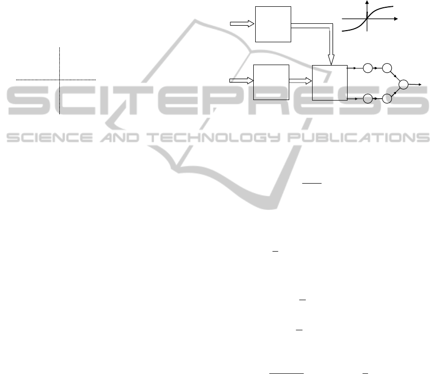
Orthogonal filter based structure of function
approximator is shown in Fig.3. To simplify the
presentation, we assume that the structure in Fig.3 is
8-dimensional, i.e. dim x = 8.
Orthogonal
Filter
weight
matrix
-W-1
v
Orthogonal
Filter
weight
matrix
W-1
u
i
x
i
x
Memory
Modules
+
.
.
c
1
c
m
z=f(x)
y
1
.
.
.
y
m
Spectrum memorizing
o
()
o
()
Pattern recognition
Spectrum analysis
of training vectors
0
0 y
(y)+
0
(y)
Figure 3: Orthogonal filter-based structure of a function
approximator.
This structure relies on using the following
kernels (Sienko and Citko, 2009):
TT
iii
2
1
0
1w
0i
K( , ) ( )
o
uv uv uv
(12)
where:
0
( . ) – a nonlinear odd function
( . ) – Kronecker’s delta
0
0
8
oi ki
k=1
1
8
w= u
, u
i
= [ u
1i
. , u
2i
, … , u
8i
]
T
Since:
ii
1
2
uW1x
(13)
1
2
vW1x
(14)
then
ij jj
TT TT
0i0i
2
0
K( , )
11
2(1 w ) 2
i
xx xWx xWx
(15)
and kernel matrix has a form:
K = K
s
+
0
1
(16)
where: K
s
- skew-symmetric matrix.
dim K
s
= m (number of training points)
It is clear that the design equation (11), with the
kernel matrix (16), is for
0
> 0 well-posed. Hence, a
numerical stable solution exists:
-1
cKz
(17)
NCTA 2011 - International Conference on Neural Computation Theory and Applications
126

Moreover, Eq.(11) can be embedded into the
following differential equation:
0
()()
s
ς
K1Θ
ς
z
(18)
and hence, for number m even (i.e. even number of
training points), it can be implemented by a lossless
neural network, as shown schematically in Fig.4.
(
) = c
z
-
0
1
Lossless neural
network
Weight matrix
W=-K
s
Figure 4: Lossless neural network-based structure for
solution of Eq.(17).
The output of this neural network is:
1
0
() ( )
s
c Θζ K1z
(19)
The stability of solution (19) can be achieved by
damping action of parameter
0
> 0 (it can be
regarded as a regularization mechanism (Evgeniou
et. al., 2000). It is easy to see that the lossless neural
network shown in Fig.4. can be realized by using
octonionic modules, similarly as Hamiltonian neural
network given by Eq.(3). Thus, one gets the
following statement: Octonionic module is a
fundamental building block for the realization of AI
compatible processors. The 8-dimensional structure
from Fig.3 can be directly scaled up to dimension
N = 2
k
, k = 5, 6, 7, … using octonionic modules.
4 ON IMPLEMENTATION OF
OCTONIONIC MODULES
It can be seen that HNN as described by Eq.(2) is a
compatible connection of n elementary building
blocks-lossless neurons. A lossless neuron is
described by the differential equation:
1
111
21 2
2
d
x0wΘ(x )
xw0Θ(x )
d
(20)
Hence, the octonionic module, with weight matrix
W
8
consists of four lossless neurons, according to
Eq.(6). A practical circuit solution of near lossless
neurons can be realized using nonlinear voltage
controlled current sources (VCCS), which are
compatible with VLSI technology. A concrete
circuit however, is beyond the scope of this
presentation.
5 CONCLUSIONS
The main goal of this paper was to prove the
following statement:
AI compatible processor should be formulated in
the form of top-down structure via the following
hierarchy: Hamiltonian neural network (composed
of lossless neurons) – octonionic module (a basic
building block) – nonlinear voltage controlled
current source (device compatible with VLSI
technology).
Hence, it has been confirmed in this paper that
by using octonionic module based structures, one
obtains regularized and stable networks for learning.
Thus, typical for AI tasks, such as realization of
classifiers, pattern recognizers and memories, could
be physically implemented for any number N=2
k
(dimension of input vectors) and any even m <
(number of training patterns).
It is clear that octonionic module cannot be
ideally realized as an orthogonal filter (decoherence-
like phenomena).
Hence, the problem under consideration now is
as follows: how exactly an octonionic module be
realized by using cheap VLSI technology to
preserve the main property-orthogonality, power
efficiency and scaleability.
The possibility to directly transform the static
structure to the phase-locked loop (PLL)-based
oscillatory structure of octonionic modules is
noteworthy.
REFERENCES
Gea-Banacloche, J., (2010). Quantum Computers: A status
update,
Proc. IEEE, vol. 98, No 12.
Hooft, G., (2000). Determinism and Dissipation in
Quantum Gravity.
arXiv: hep-th/0003005v2, 16.
Basu, A., Hasler, P. A, (2010). Nullcline-based Design of
a Silicon Neuron. Proc. IEEE Tr. on CAS, vol 57, No
11.
Versace, M., Chandler, B., (2010). The Brain of a New
Machine
. IEEE Spectrum, vol.47, No 12.
Sienko, W., Citko, W., (2009). Hamiltonian Neural
Networks Based Networks for Learning, In Mellouk,
A. and Chebira, A. (Eds.),
Machine Learning, ISBN
978-953-7619-56-1, J, pp. 75-92, Publisher: I-Tech,
Vienna, Austria.
Evgeniou, T., Pontil, M., Poggio, T., (2000).
Regularization Networks and Support Vector
Machines, In Smola, A., Bartlett, P., Schoelkopf, G.,
Schuurmans, D., (Eds),
Advances in Large Margin
Classifiers
, pp. 171-203, Cambridge, MA, MIT Press.
HAMILTONIAN NEURAL NETWORK-BASED ORTHOGONAL FILTERS - A Basis for Artificial Intelligence
127
