HYBRID RULES OF PERTURBATION

IN DIFFERENTIAL EVOLUTION FOR DYNAMIC OPTIMIZATION

Mikołaj Raciborski

, Krzysztof Trojanowski

and Piotr Kaczy´nski

Cardinal Stefan Wyszy´nski University, Faculty of Mathematics and Natural Sciences, College of Sciences, Warsaw, Poland

Institute of Computer Science, Polish Academy of Sciences, Warsaw, Poland

Keywords:

Adaptive differential evolution, Dynamic optimization, Symmetric α-stable distribution.

Abstract:

This paper studies properties of a differential evolution approach (DE) for dynamic optimization problems.

An adaptive version of DE, namely the jDE algorithm has been applied to two well known benchmarks:

Generalized Dynamic Benchmark Generator (GDBG) and Moving Peaks Benchmark (MPB) reimplemented

in a new benchmark suite

Syringa

. The main novelty of the presented research concerns application of

new type of solution, that is, solution mutated with an operator originated from another metaheuristics. The

operator uses a symmetric α-stable distribution variate for modiﬁcation of the solution coordinates.

1 INTRODUCTION

Optimization in dynamic environments is a continu-

ous subject of interest for many research groups. In

the case of dynamic optimization the algorithm has to

cope with changes in the ﬁtness landscape, i.e., in the

evaluation function parameters or even in the evalu-

ation function formula which appear during the pro-

cess of optimum search. There exists a number of dy-

namic optimization benchmarks designed to estimate

efﬁciency of optimization algorithms. Among these

benchmarks we selected two with the search space de-

ﬁned in R

to evaluate the differential evolution (DE)

approach and especially the idea of hybrid population

application. DE approach which originated with the

Genetic Annealing algorithm (Price, 1994) has been

studied from many points of view (for detailed discus-

sion see, for example, monographs (Feokistov, 2006;

Price et al., 2005)). The adaptive version of the DE

algorithm (Brest et al., 2006) differs form the basic

approach in that a self-adaptive control mechanism is

used to change the control parameters F and CR dur-

ing the run.

In the presented research we are interested in ver-

iﬁcation of the positive or negative role of a muta-

tion operator originating from another heuristic ap-

proach when it is applied in the DE algorithm. The

proposed type of mutation employs random variates

controlled by the α-stable distribution which already

proved their usefulness in other version of evolution-

ary approach and in the particle swarm optimization.

The paper is organized as follows. In Section 2

a brief description of the optimization algorithm is

presented. Section 3 discuss properties of new type

of mutation introduced to jDE. The description of a

new benchmark suite

Syringa

is given in Section 4

whereas Section 5 includes some details of the ap-

plied measure and the range of the performed tests.

Section 6 shows the results of experiments. Section 7

concludes the presented research.

2 THE jDE ALGORITHM

The differential evolution algorithm is an evolution-

ary method with a very speciﬁc mutation operator

controlled by the scale factor F. Three different, ran-

domly chosen solutions are needed to mutate a target

solution x

: a base solution x

and two difference so-

lutions x

and x

. Then, a mutant undergoes discrete

recombination with the target solution which is con-

trolled by the crossover probability factor CR ∈[0, 1].

Finally, in the selection stage trial solutions compete

with their target solutions for the place in the pop-

ulation. This strategy of population management is

called DE/rand/1/bin which means that the base solu-

tion is randomly chosen, 1 difference vector is added

to it and the crossover is based on a set of independent

decisions for each of coordinates, that is, a number of

parameters donated by the mutant closely follows a

binomial distribution.

Raciborski M., Trojanowski K. and Kaczy

nski P..

HYBRID RULES OF PERTURBATION IN DIFFERENTIAL EVOLUTION FOR DYNAMIC OPTIMIZATION.

DOI: 10.5220/0003671800320041

In Proceedings of the International Conference on Evolutionary Computation Theory and Applications (ECTA-2011), pages 32-41

ISBN: 978-989-8425-83-6

 2011 SCITEPRESS (Science and Technology Publications, Lda.)

Algorithm 1: jDE algorithm.

1: Create and initialize the reference set of (k·m) solutions

2: repeat

3: for l = 1 to k do {for each subpopulation}

4: for i = 1 to m do {for each solution in a subpopulation}

5: Select randomly three solutions: x

l,0

, x

l,1

, and x

l,2

such that: x

l,i

6= x

l,0

and x

l,1

6= x

l,2

6: for j = 1 to n do {for each dimension in a solution}

7: if (rand(0,1) > CR

l,i

) then

8: u

l,i

= x

l,0

+ F

l,i

·(x

l,1

−x

l,2

)

9: else

10: u

l,i

= x

l,i

11: end if

12: end for

13: end for

14: end for

15: for i = 1 to (k ·m) do {for each solution}

16: if ( f(u

) < f(x

) then {Let’s assume this is a minimization problem}

17: x

= u

18: end if

19: Recalculate F

and CR

20: Apply aging for x

21: end for

22: Do overlapping search

23: until the stop condition is satisﬁed

The jDE algorithm (depicted in Figure 1) extends

functionality of the basic approach in many ways.

First, each object representing a solution in the popu-

lation is extended by a couple of its personal param-

eters CR and F. They are adaptively modiﬁed every

generation (Brest et al., 2006). The next modiﬁcations

have been introduced just for better coping in the dy-

namic optimization environment. The population of

solutions has been divided into ﬁve subpopulations of

size ten. Each of them has to perform its own search

process, that is, no information is shared between sub-

populations. Every solution is a subject to the aging

procedure protecting against stagnation in local min-

ima and just the global-best solution is excluded from

this. To avoid overlapping between subpopulations a

distance between subpopulation leaders is calculated

and in the case of too close localization one of sub-

populations is reinitialized. However, as in previous

case the subpopulation with the global-best is never

the one to reinitialize. The last extension is a mem-

ory structure called archive. The archive is increased

after each change in the ﬁtness landscape by the cur-

rent global-best solution. Recalling from the archive

can be executed every reinitialization of a subpopula-

tion, however, decision about the execution depends

on a few conditions. Details of the above-mentioned

extensions can be found in (Brest et al., 2009).

3 PROPOSED EXTENSION OF

jDE

The novelty in the algorithm concerns introduction of

new type of solutions into the population of size M. A

small number of new solutions (just one, two, or three

pieces) replace the classic ones so the population size

remains the same. The difference between the classic

solutions and the new ones lies in the way they are

mutated. New type of mutation operator is based on

the rules of movement governing quantum particles in

mQSO (Trojanowski, 2009).

In the ﬁrst phase of the mutation, we generate

a new point uniformly distributed within a hyper-

sphere surrounding the mutated solution. In the sec-

ond phase, the point is shifted along the direction de-

termined by the hypersphere center and the point. The

distance d

′

from the hypersphere center to the ﬁnal lo-

cation of the point is calculated as follows:

′

= d ·SαS(0, σ) ·exp(−f

′

)), (1)

where d is a distance from the original location ob-

tained in the ﬁrst phase, SαS(·, ·) denotes a symmet-

ric α-stable distribution variate, σ is evaluated as in

eq. (2) and f

′

) as in eq. (3):

HYBRID RULES OF PERTURBATION IN DIFFERENTIAL EVOLUTION FOR DYNAMIC OPTIMIZATION

σ = r

SαS

·(D

/2) (2)

′

) =

f(x

) − f

min

( f

max

− f

min

)

(3)

where:

max

= max

j=1,...,M

f(x

), f

min

= min

j=1,...,M

f(x

The α-stable distribution (called also a Lev´y distribu-

tion) is controlled by four parameters: stability index

α (α ∈ (0,2]), skewness parameter β, scale parame-

ter σ and location parameter µ. In our case we as-

sume µ = 0 and apply the symmetric version of this

distribution (denoted by SαS for ”symmetric α-stable

distribution”), where β is set to 0.

The resulting behavior of the proposed operator is

characterized by two parameters: the parameter r

SαS

which controls the mutation strength, and the param-

eter α which determines the shape of the α-stable dis-

tribution. The solutions mutated in this way are la-

beled as s

Lev´y

in the further text.

4 THE Syringa BENCHMARK

SUITE

For the experimental research we developed a new

testing environment

Syringa

which is able to sim-

ulate behavior of a number of existing benchmarks

and to create completely new instances as well. The

structure of the

Syringa

code originates from a ﬁt-

ness landscape model where the landscape consists of

a number of simple components. A sample dynamic

landscape consists of a number of components of any

types and individually controlled by a number of pa-

rameters. Each of the components covers a subspace

of the search space. The ﬁnal landscape is the result

of a union of a collection of components such that

each of the solutions from the search space is covered

by at least one component. In the case of a solution

belonging to the intersection of a number of compo-

nents the solution value equals (1) the minimum (for

minimization problems) or (2) maximum (otherwise)

value among the values obtained for the intersected

components or (3) this can be also a sum of the ﬁt-

ness vales obtained from these components (not used

in our case). Eventually, the

Syringa

structure is a

logical consequence of the following assumptions:

1. the ﬁtness landscape consists of a number of any

different component landscapes,

2. the dynamics of each of the components can be

different and individually controlled,

3. a component can cover a part or the whole of the

search space, thus, in case of a solution covered

by more than one component the value of this so-

lution can be a minimum, a maximum or a sum of

values returned by the covering components.

4.1 The Components

The current version of

Syringa

consists of six types

of component functions (Table 1) deﬁned for the real-

valued search space. All of the formulas include

the number of the search apace dimensions n which

makes them able to deﬁne for the search spaces of

any given complexity.

There can be deﬁned a number of parameters

which individually deﬁne the component properties

and allow to introduce dynamics as well. For each

of the components we can deﬁne two groups of pa-

rameters which inﬂuence the formula of the compo-

nent ﬁtness function: the parameters from the former

one are embedded in the component function formula

whereas the parameters from the latter one control

rather the output of the formula application. For ex-

ample, when we want to stretch the landscape over the

search space each of the solution coordinates is multi-

plied by the scaling factor. For a non–uniform stretch-

ing we need to use a vector of factors containing in-

dividual values for each of the coordinates. We call

this type of modiﬁcation a horizontal scaling and this

represents the ﬁrst type of component changes. The

example of the second type is a vertical scaling where

just the ﬁtness value of a solution is multiplied by a

scaling factor. The ﬁrst group of parameters controls

changes like horizontal translation, horizontalscaling,

and rotation. For simplicity they are called horizon-

tal changes in the further text. The second group of

changes (called respectively vertical changes) is rep-

resented by vertical scaling and vertical translation.

All of the changes can be obtained by dynamic mod-

iﬁcation of respective parameters during the process

of search.

4.2 Horizontal Change Parameters

In this case the coordinates of the solution x (a vec-

tor, i.e., a matrix of size n by 1) are modiﬁed before

the component function equation is applied. The new

coordinates are obtained with the following formula:

′

= M·(W·(x+ X)) (4)

where X is a translation vector,W isa diagonal matrix

of scaling coefﬁcients for the coordinates, and M is an

orthogonal rotation matrix.

ECTA 2011 - International Conference on Evolutionary Computation Theory and Applications

Table 1:

Syringa

components.

name formula domain

Peak (F

) f(x) =

∑

j=1

[-100,100]

Cone (F

) f(x) = 1 −

∑

j=1

[-100,100]

Sphere (F

) f(x) =

∑

i=1

[-100,100]

Rastrigin (F

) f(x) =

∑

i=1

−10cos(2πx

) + 10) [-5,5]

Griewank (F

) f(x) =

4000

∑

i=1

)

−

∏

i=1

cos(

√

) + 1 [-100,100]

Ackley (F

) f(x) = −20exp(−0.2

∑

i=1

) −exp(

∑

i=1

cos(2πx

)) + 20+ e [-32,32]

4.3 Vertical Change Parameters

Changes of the ﬁtness function value are executed ac-

cording to the following formula:

′

(x) = f(x) ·v+ h (5)

where v is a vertical scaling coefﬁcient and h is a ver-

tical translation coefﬁcient.

4.4 Parameters Control

In the case of dynamic optimization the ﬁtness land-

scape components has to change the values of their

parameters during the process of search. There were

deﬁned four different characteristics of variability

which were applied to the component parameters:

small step change (T

— eq. (6)), large step change

— eq. (7)), and two versions of random changes

— eq. (8) and T

— eq. (9)). The change ∆ of a

parameter value is calculated as follows:

∆ = α·r·(max−min); α = 0.04, r = U(0, 1), (6)

∆ = (α·sign(r

) + (α

max

−α) ·r

) ·(max−min);

α = 0.04, r

1,2

= U(0, 1), α

max

= 0.1 (7)

∆ = N(0,1) (8)

∆ = U(r

min

max

) (9)

In the above-mentioned equations max and min rep-

resent upper and lower boundary of the search space,

N(0,1) is a random value obtained with gaussian dis-

tribution where µ = 0 and σ = 1, U(0, 1) is a ran-

dom value obtained with uniform distribution form

the range [0,1], and [r

min

max

] deﬁne the feasible

range of ∆ values.

The model of

Syringa

assumes that the compo-

nent parameter control is separated from the compo-

nent, that is, a dynamic component has to consist of

two objects: the ﬁrst one represents an evaluator of

solutions (i.e., a component of any type mentioned in

Table 1) and the second one is an agent which con-

trols the behavior of the evaluator. The agent deﬁnes

initial set of values for the evaluator parameters and

during the process of search the values are updated by

the agent according to the assumed characteristic of

variability. Properties of all the types of components

are uniﬁed so as to make possible assignment of any

agent to any component. This architecture allows to

create multiple classes of dynamic landscapes.

In the presented research we started with simu-

lation of two existing benchmarks: Generalized Dy-

namic Benchmark Generator (GDBG) (Li and Yang,

2008) and the Moving Peaks Benchmark genera-

tor (Branke, 1999). In both cases optimization is

carried out in a real-valued multidimensional search

space, and the ﬁtness landscape is built of multiple

component functions controlled individually by their

parameters. For appropriate simulation of any of the

two benchmarks there are just two things to do: select

a set of the right components and build agents which

will control the components in the same manner like

in the original benchmarks.

4.5 Simulation of Moving Peaks

Benchmark (MPB)

In the case of MPB, three scenarios of the benchmark

parameters control are deﬁned (Branke, 1999). We

did experiments for the ﬁrst and the second scenario.

The selected ﬁtness landscape consists of a set of

peaks (F

— the ﬁrst scenario) or cones (F

— the sec-

ond scenario) which undergo two types of horizontal

changes: the translation and the scaling and just one

vertical change, that is, the translation. The horizon-

tal scaling operator has the same scale coefﬁcient for

each of the dimensions, so in this speciﬁc case this co-

efﬁcient is represented as a one-dimensional variable

w instead of the vector W.

The parameters X, w and v are embedded into the

HYBRID RULES OF PERTURBATION IN DIFFERENTIAL EVOLUTION FOR DYNAMIC OPTIMIZATION

peak function formula f(x) in the following way:

peak

(x) =

1+ w·

∑

j=1

−X

)

(10)

The parameters X, w and h are embedded into the

cone function formula f(x) in the following way:

cone

(x) = h −w·

∑

j=1

−X

)

(11)

All the modiﬁcations of the component parame-

ters belong to the fourth characteristic of variability

where for every change r

min

and r

max

are rede-

ﬁned in the way to keep the value of each modiﬁed

parameter in the predeﬁned interval of feasible val-

ues. Simply, for every modiﬁed parameter of transla-

tion or scaling, which can be represented as a symbol

p: r

min

= p

min

− p and r

max

= p

max

− p. For the hor-

izontal scaling the interval is set to [1;12] and for the

vertical scaling — to [30;70]. For the horizontal trans-

lation there is a constraint for the euclidean length of

the translation: |X|≤3. For both scenarios in the ﬁrst

version there are ten moving components whereas in

the second version 50 moving components is in use.

4.6 Simulation of Generalized Dynamic

Benchmark Generator (GDBG)

GDBG consists of two different benchmarks:

Dynamic Rotation Peak Benchmark Generator

(DRPBG) and Dynamic Composition Benchmark

Generator (DCBG). There are ﬁve types of com-

ponent functions: peak (F

), sphere (F

), Rastrigin

), Griewank (F

), and Ackley (F

). F

is the base

component for DRPBG whereas all the remaining

types are employed in DCBG.

4.6.1 Dynamic Rotation Peak Benchmark

Generator (DRPBG)

There are four types of the component parameter

modiﬁcation applied in DRPBG: horizontal transla-

tion, scaling and rotation and vertical scaling. As in

the case of MPB the horizontal scaling operator has

the same scale coefﬁcient for each of the dimensions,

so in this speciﬁc case this coefﬁcient is also repre-

sented as a one-dimensional variable w instead of the

vector W. The component function formula is the

same as in the eq. (10).

Values of the translation vector X in subsequent

changes are evaluated with use of the rotation ma-

trix M. Clearly, we apply the rotation matrix to the

current coordinates of the component function opti-

mum o, that is: o(t + 1) = o(t) · M(t) (where t is

the number of the current change in the component)

and then the ﬁnal value of X(t + 1) is calculated:

X(t + 1) = o(t + 1) −o(0).

Subsequent values of the horizontal scaling pa-

rameter w and the vertical scaling parameter v are

evaluated according to the ﬁrst, the second or the third

characteristic of variability, that is, T

, T

or T

For every change a new rotation matrix M is gen-

erated which is common for all the components. The

rotation matrix M is obtained as a result of multipli-

cation of a number of rotation matrices R where each

of R represents rotation in just one plane of the multi-

dimensional search space.

In DRPBG we start with a selection of the rotation

planes, that is, we need to generate a vector r of size

l where l is an even number and l ≤ n/2. The vec-

tor contains randomly selected search space dimen-

sion identiﬁers without repetition. Then for each of

the planes deﬁned in r by subsequent pairs of indices:

[1,2], [3,4], [5,6], .. . [l −1,l] their rotation angles are

randomly generated and ﬁnally respective matrices

r[1],r[2]

,... R

r[l− 1],r[l]

are calculated (R

(θ) represents

rotation by the θ angle along the plane i–j) (c.f. (Sa-

lomon, 1996)). Eventually, the rotation matrix M is

calculated as follows:

M(t) = R

r[1],r[2]

(θ(t))···R

r[l− 1],r[l]

(θ(t)). (12)

Syringa

the method of the rotation matrix gen-

eration slightly differs from the one described above.

Instead of the vector r there is a vector Θ which repre-

sents a sequence of rotation angles for all the possible

planes in the search space. The position in the vector

Θ deﬁnes the rotation plane. Simply, Θ(1) represents

the plane [1,2], Θ(2) represents the plane [2,3] and

so on until the plane [n-1,n]. Then there go planes

created from every second dimensions, that is, [1,3],

[2,4] and so on until the plane [n-2,n]. Then there

go planes created from every third dimensions, then

those created from every fourth, and so on until there

appears the last plane created from the ﬁrst and the

last dimension. When Θ(i) equals zero this means,

that there is no rotation for the i-th plane, otherwise

the respective rotation matrix R is generated. The ﬁ-

nal stage of generation of the matrix M is the same

as in the description above, that is, the rotation matrix

M is the result of multiplication of all the matrices R

generated from the vector Θ.

Finally, it is important to note that in the above

description the matrix M has been used twice for the

evaluation of the component modiﬁcation parameters:

the ﬁrst time when the translation vector X is calcu-

lated and the second time when the rotation is applied,

that is, just before the application of the equation (10).

ECTA 2011 - International Conference on Evolutionary Computation Theory and Applications

4.6.2 Dynamic Composition Benchmark

Generator (DCBG)

DCBG performs ﬁve types of the component param-

eter modiﬁcation: horizontal translation, scaling and

rotation and vertical translation and scaling. The re-

spective parameters are embedded into the function

formula f”(x) in the following way (Liang et al.,

2005; Suganthan et al., 2005):

f”(x) = (v·( f

′

(M·(W·(x+ X))) + h)) (13)

where:

v is the weight coefﬁcient depending of the

currently evaluated x,

W is called a stretch factor which equals 1

when the search range of f(x) is the same as

the entire search space and grows when the

search range of f(x) decreases,

′

(x) represent the value of f(x) normalized

in the following way: f

′

(x) = C · f(x)/|f

max

where the constant C = 2000 and f

max

the estimated maximum value of function f

which is one of the four: sphere (F

), Rastri-

gin (F

), Griewank (F

), or Ackley (F

Syringa

the properties of some of the parame-

ters has had to be changed. The ﬁrst difference is in

the evaluation of the weight coefﬁcient v which due to

the structure of the assumed model cannot depend of

the currently evaluated x. Therefore, we assumed that

v = 1. There is also no scaling, i.e., W is an identity

matrix because we assumed that the component func-

tions are always deﬁned for the entire search space.

The last issue is about the rotation matrix M which is

calculated in the same way as for the

Syringa

version

of DRPBG. Eventually, the

Syringa

version of f”(x)

has the following shape:

f”(x) = (( f

′

(M·((x+ X))) + h)) (14)

Thus, the

Syringa

version of DCBG differs from

the original one because it does not contain the hor-

izontal scaling, the rotation matrix M is evaluated in

the different way and the stretch factor always equals

one. However, a kind of the vertical scaling is still

present and can be found in the step of the f (x) nor-

malization.

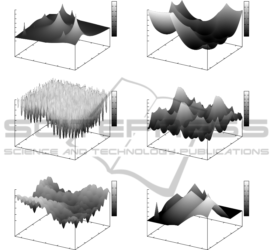
Fitness landscapes of the selected benchmark in-

stances generated for two-dimensional search space

are depicted in Figure 1. Please note that the land-

scape generated by DRPBG with ten peak compo-

nents is in fact exactly the same as the one which

would be generated by MPB sc.1 with ten peak com-

ponents since in both cases the same component func-

tion is in use. Of course the dynamics of the two

benchmark instances is different so there is no chance

for duplication of the experiments.

5 PLAN OF EXPERIMENTS

5.1 Performance Measure

For comparisons between the results obtained for dif-

ferent benchmark instances and different versions of

the algorithms the ofﬂine error (Branke, 1999)(brieﬂy

oe) was selected. The measure represents the aver-

age deviation from the optimum of the best individual

value since the last change in the ﬁtness landscape.

Formally:

oe =

changes

∑

j=1

( j)

∑

i=1

( f(x

∗j

) − f(x

best

))

(15)

where N

( j) is a total number of solution evaluations

performed for the j-th static state of the landscape,

f(x

∗j

) is the value of an optimal solution for the j-th

landscape and f(x

best

) is the current best value found

for the j-th landscape. It should be clear that the mea-

sure oe should be minimized, that is, the better result

the smaller the value of oe.

Our algorithm has no embedded strategy for de-

tecting changes in the ﬁtness landscapes. Simply,

the last step in the main loop of the algorithm exe-

cutes the reevaluation of the entire current solution

set. Therefore, our optimization system is informed

of the change as soon as it occurs, and no additional

computational effort for its detection is needed.

5.2 The Tests

We performed experiments with a subset of GDBG

benchmark functions as well as with four versions of

MPB. For each of the components there is a deﬁned

feasible domain which, unfortunately, is not the same

in every case (see the last column in Table 1). For

this reason the boundaries for the search space dimen-

sions in the test-cases are not the same but adjusted re-

spectively to the components. For GDBG the feasible

search space is within the hypercube with the same

boundaries for each dimension, namely [−7.1,7.1]

whereas for MPB — [−50,50]. These box constraints

mean that both solutions and components should not

leave this area during the entire optimization process.

The number of ﬁtness function evaluations be-

tween subsequent changes was calculated according

to the rules as in the CEC’09 competition, that is,

for 10

·n ﬁtness function calls between subsequent

changes where n is a number of search space dimen-

sions and in this speciﬁc case n equals ﬁve for all of

the benchmark instances.

To decrease the number of algorithm conﬁgura-

tions which would be experimentally veriﬁed we de-

HYBRID RULES OF PERTURBATION IN DIFFERENTIAL EVOLUTION FOR DYNAMIC OPTIMIZATION

-4

-2

-4

-2

-4

-2

-4

-2

5000

10000

15000

20000

25000

30000

5000

10000

15000

20000

25000

30000

-4

-2

-4

-2

5000

10000

15000

20000

25000

30000

5000

10000

15000

20000

25000

30000

-4

-2

-4

-2

200

400

600

800

1000

1200

1400

1600

1800

200

400

600

800

1000

1200

1400

1600

1800

-4

-2

-4

-2

5000

10000

15000

20000

25000

5000

10000

15000

20000

25000

-40

-20

-40

-20

Figure 1: Fitness landscapes of the benchmark instances for 2D search space: DRPBG with ten peak components and DCBG

with ten sphere components (ﬁrst row), DCBG with ten Rastrigin components and DCBG with ten Griewank components

(second row), DCBG with ten Ackley components and MPB sc. 2 with ten cones (the last row).

cided to ﬁx the value of the parameter r

SαS

and the

only varied parameter was α. In the preliminary

phase of experimental research we tested efﬁciency

of the algorithm for different values of r

SαS

and ana-

lyzed obtained values of error. Eventually, for GDBG

SαS

= 0.6 whereas for MPB it is ten times smaller,

that is, r

SαS

= 0.06. Thus, for each of the benchmark

instances there were performed just 32 experiments:

for α between 0.25 and 2 varying with step 0.25 and

for 0, 1, 2 and 3 solutions of new type present in the

population. For each of the conﬁgurations the experi-

ments were repeated 20 times and each of them con-

sisted of 60 changes in the ﬁtness landscape. Graphs

and tables present mean values of oe calculated for

these series.

6 THE RESULTS

The best values of ofﬂine error obtained for each of

the benchmarkinstances are presented in Table 2. The

table contains names of the instances, the mutation

parameter conﬁgurations (i.e. values of α and ind

SαS

)

and the mean values of oe. The instances are sorted in

ascending order of obtained oe values (more or less).

This way we can easily show which of the instances

ECTA 2011 - International Conference on Evolutionary Computation Theory and Applications

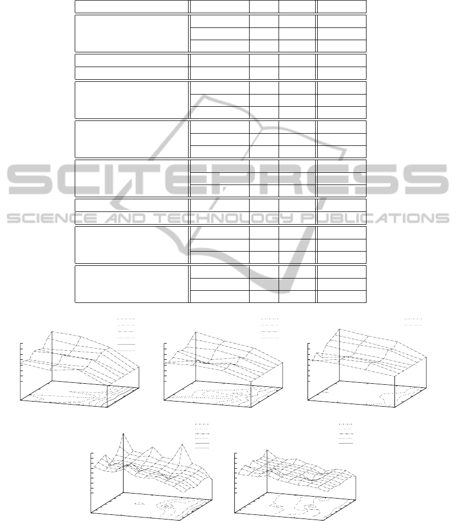
Table 2: The least ofﬂine error (oe) mean values obtained for all the benchmark instances; the instances are sorted in ascending

order of oe; for each of the instances three values are presented for three change types of the GDBG control parameters: T

and T

(except for MPB where there are two cases: with ten and 50 peaks/cones).

the benchmark instance change type α ind

SαS

1.25 3.00 0.16813

(Griewank) T

1.50 3.00 0.13977

2.00 3.00 0.35606

MPB sc. 1 with ten peaks 1.00 1.00 0.35622

MPB sc. 1 with 50 peaks 1.50 1.00 0.66492

DCBG with F

1.50 2.00 1.22583

(sphere components) T

0.75 1.00 1.81625

1.75 3.00 5.32476

DRPBG with ten F

2.00 1.00 1.98783

1.00 1.00 2.51758

0.50 1.00 3.76098

DRPBG with 50 F

1.25 1.00 3.35855

1.00 1.00 4.24594

0.75 1.00 5.87459

MPB sc. 2 with ten cones — 0.00 4.11117

MPB sc. 2 with 50 cones 0.50 1.00 3.74856

DCBG with F

2.00 1.00 8.41941

(Ackley components) T

1.50 1.00 9.77345

1.50 1.00 14.24450

DCBG with F

— 0.00 570.72

(Rastrigin components) T

— 0.00 610.565

— 0.00 661.395

0.5

1.5

550

600

650

700

750

800

850

900

700

675

650

625

600

575

ind

S α S

0.5

1.5

550

600

650

700

750

800

850

900

700

675

650

625

ind

S α S

0.5

1.5

550

600

650

700

750

800

850

900

700

675

ind

S α S

0.25

0.5

0.75

1.25

1.5

1.75

6.5

5.5

4.5

ind

S α S

0.25

0.5

0.75

1.25

1.5

1.75

4.5

5.5

6.5

7.5

5.5

5.25

4.75

4.5

ind

S α S

Figure 2: Characteristics of oe for jDE: the cases where hybrid solution deteriorates the results, i.e., DCBG with F

(Rastrigin

components) (the ﬁrst row) and MPB sc.2 with 10 and 50 F

(cones) (the second row); the subsequent graphs in the ﬁrst row

represent three change types of the GDBG control parameters: T

, T

and T

were the most difﬁcult and which were the easiest.

All the results are depicted in Figures 2 and 3. The

graphs are divided into two groups: where due to the

presence of s

Lev´y

solutions obtained results deterio-

HYBRID RULES OF PERTURBATION IN DIFFERENTIAL EVOLUTION FOR DYNAMIC OPTIMIZATION

0.5

1.5

0.1

0.12

0.14

0.16

0.18

0.2

0.22

0.24

0.26

0.28

0.3

0.2

0.18

ind

S α S

0.5

1.5

0.1

0.12

0.14

0.16

0.18

0.2

0.22

0.24

0.26

0.28

0.3

0.2

0.18

0.16

0.14

ind

S α S

0.5

1.5

0.3

0.4

0.5

0.6

0.7

0.8

0.5

0.45

0.4

ind

S α S

0.25

0.5

0.75

1.25

1.5

1.75

0.3

0.35

0.4

0.45

0.5

0.55

0.6

0.65

0.7

0.55

0.5

0.45

0.4

ind

S α S

0.25

0.5

0.75

1.25

1.5

1.75

0.5

0.6

0.7

0.8

0.9

1.1

0.8

0.75

0.7

ind

S α S

0.5

1.5

2.5

3.5

1.75

1.5

1.25

ind

S α S

0.5

1.5

2.5

3.5

ind

S α S

0.5

1.5

5.5

6.5

7.5

8.5

6.5

6.25

5.75

5.5

ind

S α S

0.5

1.5

4.5

3.5

2.5

ind

S α S

0.5

1.5

4.5

3.5

ind

S α S

0.5

1.5

6.5

5.5

4.5

3.5

ind

S α S

0.5

1.5

5.5

4.5

3.5

ind

S α S

0.5

1.5

5.5

4.5

ind

S α S

0.5

1.5

7.5

6.5

ind

S α S

0.5

1.5

ind

S α S

0.5

1.5

ind

S α S

0.5

1.5

ind

S α S

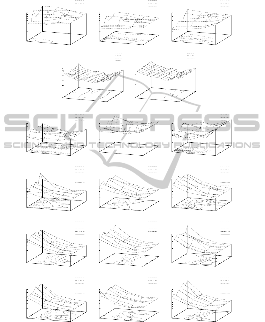
Figure 3: Characteristics of oe for jDE: the cases where hybrid solution improves the results: DCBG with F

(Griewank

components) (the ﬁrst row), MPB sc.1 with ten and with 50 F

(peaks) (the second row) DCBG with F

(sphere components)

(the third row), DRPBG with ten and with 50 F

(peaks) (the fourth and the ﬁfth row), DCBG with F

(Ackley components)

(the last row); the columns represent three change types of the GDBG control parameters: T

, T

and T

(except for MPB

where there are just two cases: with ten and 50 peaks).

ECTA 2011 - International Conference on Evolutionary Computation Theory and Applications

rated (Figure 2), and where application of s

Lev´y

solu-

tions in the population improved the results, that is,

obtained error decreased (Figure 3).

For each of the benchmark instances there were

obtained 32 values of oe which are presented in a

graphicalform as a surface generated for different val-

ues of the number of s

Lev´y

solutions (that is, ind

SαS

)

and α. The benchmark instances in the Figures are

ordered in the same way as in Table 2.

7 CONCLUSIONS

In this paper we introduce hybrid structure of popula-

tion in differential evolution algorithm jDE and study

its properties when applied to dynamic optimization

tasks. This is a case of a kind of technology trans-

fer where promising mechanisms form one heuris-

tic approach appear to be useful in another. The re-

sults show that mutation operator using random vari-

ates based on α-stable distribution, that is, the oper-

ator where both ﬁne local modiﬁcation and macro-

jumps can appear, improves the values of oe. Lack

of improvement appeared in two cases, that is, for

the DCBG with F4 (Rastrigin components) which is a

very difﬁcult landscape looking like a hedgehog (Fig-

ure 1, the graph in the second row on the left) and for

the MPB sc.2 with ten cones. In both cases macro-

mutation most probably introduces unnecessary noise

rather than a chance for exploration of a new promis-

ing area. Difﬁculty of the former benchmark instance

is conﬁrmed by extremely high values of error ob-

tained for all three types of change.

In the remaining cases the inﬂuence of s

Lev´y

solu-

tion presence is positive, however, it must be stressed

that the number of these solutions should be small. In

most cases the best results were obtained for just one

piece. The exception is the DCBG with F5 (Grievank

components) which was the easiest landscape for the

algorithm, easier even than the landscape build of the

spheres. In the case of the DCBG with F5 the higher

number of s

Lev´y

, the smaller value of oe.

Finally, it is worth to stress that the different com-

plexity of the tested instances shows also that when

we take them as a suite of tests and evaluate over-

all gain of the algorithm we need to apply different

weight for the successes obtained for each of the in-

stances. Simply, an improvement of efﬁciency ob-

tained for DCBG with Grievank components havedif-

ferent signiﬁcance than the same improvement for,

e.g., DCBG with Ackley components.

REFERENCES

Branke, J. (1999). Memory enhanced evolutionary algo-

rithm for changing optimization problems. In Proc. of

the Congr. on Evolutionary Computation, volume 3,

pages 1875–1882. IEEE Press, Piscataway, NJ.

Brest, J., Greiner, S., Boskovic, B., Mernik, M., and Zumer,

V. (2006). Self-adapting control parameters in dif-

ferential evolution: A comparative study on numeri-

cal benchmark problems. IEEE Trans. Evol. Comput.,

10(6):646–657.

Brest, J., Zamuda, A., Boskovic, B., Maucec, M. S., and

Zumer, V. (2009). Dynamic optimization using self-

adaptive differential evolution. In IEEE Congr. on

Evolutionary Computation, pages 415–422. IEEE.

Feokistov, V. (2006). Differential Evolution, In Search of

Solutions, volume 5 of Optimization and Its Applica-

tions. Springer.

Li, C. and Yang, S. (2008). A generalized approach to con-

struct benchmark problems for dynamic optimization.

In Simulated Evolution and Learning, SEAL, volume

5361 of LNCS, pages 391–400. Springer.

Liang, J. J., Suganthan, P. N., and Deb, K. (2005). Novel

composition test functions for numerical global opti-

mization. In IEEE Swarm Intelligence Symposium,

pages 68–75, Pasadena, CA, USA.

Price, K. V. (1994). Genetic annealing. Dr. Dobb’s Journal,

pages 127–132.

Price, K. V., Storn, R. M., and Lampinen, J. A. (2005). Dif-

ferential Evolution, A Practical Approach to Global

Optimization. Natural Computing Series. Springer.

Salomon, R. (1996). Reevaluating genetic algorithm perfor-

mance under coordinate rotation of benchmark func-

tions. BioSystems, 39(3):263–278.

Suganthan, P. N., Hansen, N., Liang, J. J., Deb, K., Chen,

Y.-P., Auger, A., and Tiwari, S. (2005). Problem deﬁ-

nitions and evaluation criteria for the cec 2005 special

session on real-parameter optimization. Technical re-

port, Nanyang Technological University, Singapore.

Trojanowski, K. (2009). Properties of quantum particles in

multi-swarms for dynamic optimization. Fundamenta

Informaticae, 95(2-3):349–380.

HYBRID RULES OF PERTURBATION IN DIFFERENTIAL EVOLUTION FOR DYNAMIC OPTIMIZATION