INDIVIDUALLY AND COLLECTIVELY TREATED NEURONS

AND ITS APPLICATION TO SOM

Ryotaro Kamimura

IT Education Center, Tokai University, 1117 Kitakaname, Hiratsuka, Kanagawa 258-1292, Japan

Keywords:

Individually treated neurons, Collectively treated nerons, Information-theoretic learning, Free enrgy, SOM.

Abstract:

In this paper, we propose a new type of information-theoretic method to interact individually treated neurons

with collectively treated neurons. The interaction is determined by the interaction parameter α. As the param-

eter α is increased, the effect of collectiveness is larger. On the other hand, when the parameter α is smaller,

the effect of individuality becomes dominant. We applied this method to the self-organizing maps in which

much attention has been paid to the collectiveness of neurons. This biased attention has, in our view, shown

difﬁculty in interpreting ﬁnal SOM knowledge. We conducted an preliminary experiment in which the Iono-

sphere data from the machine learning database was analyzed. Experimental results conﬁrmed that improved

performance could be obtained by controlling the interaction of individuality with collectiveness. In particular,

the trustworthiness and continuity are gradually increased by making the parameter α larger. In addition, the

class boundaries become sharper by using the interaction.

1 INTRODUCTION

Neurons in neural networks have been treated indi-

vidually or collectively in different learning methods.

No attempts have been made to examine the interac-

tion of individuality with collectiveness. In this paper,

we postulate that neurons should be treated individu-

ally and collectively and these two types of neurons

should interact with each other to have special effect

for neural learning. We, in particular, focus upon the

self-organizing maps (SOM) (Kohonen, 1988), (Ko-

honen, 1995). Because only the collectiveness of neu-

rons has been taken into account in the SOM, ignoring

the properties of individual treated neurons. Thus, it

is easy to demonstrate the effect of interaction using

the SOM.

The SOM is a well-known technique for the vec-

tor quantization and the vector projection from high

dimensional input spaces into low dimensional out-

put spaces. However, it is hard to interpret ﬁnal SOM

knowledge from simple visual inspection. Thus,

many different types of visualization techniques have

been proposed, for example, the U-matrix and its vari-

ants (Ultsch, 2003b), (Ultsch, 2003a) visualization of

component planes (Vesanto, 1999), linear and non-

linear dimensionality reduction methods such as the

principal component analysis (PCA) (Bishop, 1995),

Sammon Map (Sammon, 1969) and many non-linear

methods (Joshua B. Tenenbaum and Langford, 2000),

(Roweis and Saul, 2000), (Demartines and Herault,

1997), and the responses to data samples (Vesanto,

1999). Recently, more advanced visualization tech-

niques were proposed such as gradient ﬁeld and bor-

derline visualization techniques (Georg Polzlbauer

and Rauber, 2006), the connectivity matrix of proto-

type vectors (Tasdemir and Merenyi, 2009) and the

gradient-based SOM matrix (Costa, 2010) and so on.

Even using these visualization techniques, it re-

mains to be difﬁcult to interpret ﬁnal SOM knowl-

edge. The detection of class or cluster boundaries is,

in particular, a serious problem. If neurons on both

sides of class boundaries should behave differently, it

is easy to ﬁnd the boundaries with some visualization

techniques. However, cooperation processes in SOM

diminishes the effect of the boundaries, because the

cooperation processes aim to increase continuity over

the output space. Intuitively, the continuity is contra-

dictory to the boundaries. In the proposed method,

the individuality as well as collectiveness of neurons

is introduced. The introduction of individuality is re-

lated to the more explicit detection of class boundaries

by reducing collectiveness.

Kamimura R..

INDIVIDUALLY AND COLLECTIVELY TREATED NEURONS AND ITS APPLICATION TO SOM.

DOI: 10.5220/0003677300240030

In Proceedings of the International Conference on Neural Computation Theory and Applications (NCTA-2011), pages 24-30

ISBN: 978-989-8425-84-3

 2011 SCITEPRESS (Science and Technology Publications, Lda.)

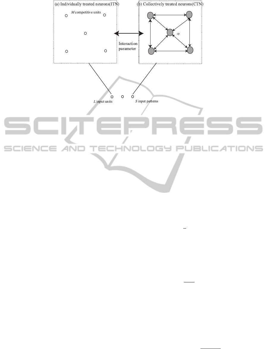
Figure 1: Concept of interaction of individuality with collectivenss.

2 THEORY AND

COMPUTATIONAL METHODS

2.1 Interaction

The individuality and collectiveness are easily im-

plemented in neural network architecture. Figure 1

shows a concept of neurons individually and collec-

tively treated. Neurons are treated individually in Fig-

ure 1(a), and collectively in Figure 1(b). Two types of

neurons are mediated by the interaction parameter α.

In our view, in the conventional SOM, neurons have

been treated collectively or cooperatively. Little atten-

tion has been paid to the individuality of neurons. For

example, the good performance of the self-organizing

maps has been evaluated by the trustworthiness and

continuity on the output and input space (Kiviluoto,

1996), (Villmann et al., 1997), (Bauer and Pawelzik,

1992), (Kaski et al., 2003), (Venna and Kaski, 2001),

(Polzlbauer, 2004), (Lee and Verleysen, 2008). No

attempts have been made to evaluate the good perfor-

mance of the self-organizing maps on the clarity of

the obtained class structure.

The individuality and collectives can be consid-

ered in terms of neighborhood functions. As the range

of the neighbors becomes smaller, the individuality

can be considered. However, those neighborhood

functions are only used for making cooperation pro-

cesses smooth. Thus, we think that it is necessary

to control or reduce the effect of cooperation among

neurons, and much more attention should be paid to

the extraction of explicit class boundaries.

2.2 ITN

When each neuron is individually treated, we can ob-

tain individually treated neurons (ITN) as shown in

Figure 1(a). In actual implementation, the method

corresponds to our information-theoretic competi-

tive learning (Kamimura et al., 2001a), (Kamimura,

2003). In this method, competition processes are sup-

posed to be realized by maximizing mutual informa-

tion between competitive units and input patterns.

Let us compute mutual information for a network

shown in Figure 1(a). The jth competitive unit output

can be computed by

∝ exp

{

−

− w

)

Λ(x

− w

)

}

, (1)

where x

and w

are supposed to represent L-

dimensional input and weight column vectors, where

L denotes the number of input units. The L ×L matrix

Λ is called a ”scaling matrix,” and the klth element of

the matrix denoted by (Λ)

is deﬁned by

(Λ)

= δ

p(k)

, k, l = 1, 2, · · · ,L. (2)

where σ is a spread parameter, and p(k) shows a ﬁr-

ing probability of the kth input unit and is initially set

to 1/L, because we have no preference in input units.

The output is increased when connection weights be-

come closer to input patterns. The conditional prob-

ability of the ﬁring of the jth competitive unit, given

the sth input pattern, can be obtained by

p( j | s) =

∑

m−1

. (3)

The probability of the ﬁring of the jth competitive

unit is computed by

INDIVIDUALLY AND COLLECTIVELY TREATED NEURONS AND ITS APPLICATION TO SOM

p( j) =

∑

s=1

p(s)p( j | s). (4)

With these probabilities, we can compute mutual in-

formation between competitive units and input pat-

terns (Kamimura et al., 2001b). Mutual information

is deﬁned by

MI =

∑

s=1

∑

j=1

p(s)p( j | s) log

p( j | s)

p( j)

. (5)

When this mutual information is maximized, just one

competitive unit ﬁres, while all the other competitive

units cease to do so. Finally, we should note that one

of the main properties of this mutual information is

that it is dependent upon the scaling matrix, or more

concretely, the spread parameter σ. As the spread pa-

rameter is decreased, the mutual information between

competitive units and input patterns tends to be in-

creased.

We can differentiate the mutual information and

obtain update rules, but direct computation of mutual

information is accompanied by computational com-

plexity (Kamimura et al., 2001a), (Kamimura, 2003).

To simplify the computation, we introduce free en-

ergy (Rose et al., 1990). The free energy F can be

deﬁned by

F = −2σ

∑

s=1

p(s)log

∑

j=1

p( j)

×exp

{

−

− w

)

Λ(x

− w

)

}

. (6)

We suppose the following equation

∗

( j | s) =

p( j)v

∑

m=1

p(m)v

. (7)

Then, the free energy can be expanded as

F =

∑

s=1

p(s)

∑

j=1

∗

( j | s)∥x

− w

∥

+2σ

∑

s=1

p(s)

∑

j=1

∗

( j | s) log

∗

( j | s)

∗

( j)

.(8)

This equation shows that, by minimizing the free en-

ergy, we can decrease mutual information as well as

quantization errors. We usually set p( j) into 1/M for

simpliﬁcation, and then

∗

( j | s) =

∑

m=1

. (9)

By differentiating the free energy, we have

∑

s=1

∗

( j | s)x

∑

s=1

∗

( j | s)

. (10)

2.3 CTN

We can extend the information-theoretic competitive

learning to a case where the collectiveness of neurons

is taken into account. For the CTN, we try to borrow

the computational methods developed for the conven-

tional self-organizing maps, and then we use the ordi-

nary neighborhood kernel used for SOM, namely,

∝ exp

(

−∥r

− r

∥

)

, (11)

where r

and r

denote the position of the jth and the

cth unit on the output space. Because the adjustment

of individuality and collectiveness, namely, neighbor-

hood relations, are realized by the interaction. The

neighborhood function has no parameters to be ad-

justed.

The collective outputs can be deﬁned by the sum-

mation of all neighboring competitive units

∝

∑

c=1

exp

{

−

− w

)

ctn

− w

)

}

(12)

where the klth element of the scaling matrix (Λ

ctn

)

is given by

(Λ

ctn

)

= δ

p(k)

ctn

, (13)

where σ

ctn

denotes the spread parameter for the col-

lective neurons. The conditional probability of the ﬁr-

ing of the j th competitive unit, given the sth input pat-

tern, can be obtained by

q( j | s) =

∑

m=1

. (14)

Thus, we must decrease the following KL divergence

measure

∑

s=1

∑

j=1

p(s)p( j | s) log

p( j | s)

q( j | s)

. (15)

As already mentioned in the above section, instead

of the direct differentiation, we introduce the free en-

ergy. The free energy can be deﬁned by

F = −2σ

∑

s=1

p(s)log

∑

j=1

q( j|s)

×exp

{

−

− w

)

Λ(x

− w

)

}

.(16)

Then, the free energy can be expanded as

NCTA 2011 - International Conference on Neural Computation Theory and Applications

F =

∑

s=1

p(s)

∑

j=1

∗

( j | s)∥x

− w

∥

+2σ

∑

s=1

p(s)

∑

j=1

∗

( j | s)

×log

∗

( j | s)

q( j | s)

, (17)

where

∗

( j | s) =

q( j | s)v

∑

m=1

q(m | s)v

. (18)

By differentiating the free energy, we can have update

rules

∑

s=1

∗

( j | s)x

∑

s=1

∗

( j | s)

. (19)

2.4 Interaction Procedures

In the interaction ITN with CTN, all neurons com-

pete with other, because our method is based upon

information-theoretic competitive learning. The de-

gree of competition is determined by the spread pa-

rameter σ and σ

ctn

for ITN and CTN. The spread pa-

rameter σ

ctn

is computed by the competition parame-

ter β

ctn

, (20)

where β is larger than zero. As the competition pa-

rameter β is larger, competition among neurons be-

comes stronger.

The spread parameter σ is gradually decreased

from β to a point by the interaction parameter α to

control ITN and CTN. For simplicity’s sake, we sup-

pose that ﬁnally the spread parameter σ is propor-

tional to the other parameter σ

ctn

. Then, we have a

relation

σ = ασ

ctn

, (21)

where α is supposed to be greater than zero. As the

interaction parameter α is larger, the spread parameter

for ITN is larger. This means that the effect of ITN

diminishes and that of CTN augments. Actually, the

spread parameter σ is decreased from the value of β

to ασ

ctn

3 RESULTS AND DISCUSSION

3.1 Experimental Setting

We present experimental results on the Ionosphere

Table 1: Quantization (QE), topographic (TE), training and

generalization (gene) errors by the conventional SOM and

the interaction method when the interaction parameter α is

changed from one to ﬁfty.

QE TE Training Gene

SOM 0.130 0.009 0.209 0.205

1 0.075 0.496 0.068 0.154

10 0.107 0.051 0.137 0.128

20 0.124 0.000 0.261 0.188

30 0.126 0.004 0.218 0.179

40 0.126 0.000 0.218 0.179

50 0.126 0.004 0.218 0.179

data from the machine learning database

to show

how well our method performs. We use the SOM

toolbox developed by Vesanto et al. (Vesanto et al.,

2000), because it is easy to reproduce the ﬁnal re-

sults presented in this paper by using this package.

In the SOM, the Batch method is used, which has

shown better performance than the popular real-time

method in terms of visualization, quantization and to-

pographic errors. To evaluate the validity of the ﬁnal

results, we tried to use the very conventional meth-

ods as well as modern methods for exact compari-

son. In the conventional methods, we used two types

of errors, namely, quantization and topographic er-

rors. The quantization error is simply the average

distance from each data vector to its BMU (best-

matching unit). The topographic error is the per-

centage of data vectors for which the BMU and the

second-BMU are not neighboring units (Kiviluoto,

1996). For more modern techniques, we used trust-

worthiness and continuity (Venna and Kaski, 2001),

(Venna, 2007) based upon the random method pro-

posed by (Kiviluoto, 1996). In addition, we computed

the error rate for training and testing data. The error

rate was computed by using the k-nearest neighbor

(k=1). For computing the generalization performance

in the error rate, we divided the data into training (2/3)

and testing (1/3) data.

3.2 Ionosphere Data

We applied the method to the ionosphere data from

the machine learning database. This radar data was

collected by a system in Goose Bay, Labrador. The

data should be classiﬁed into ”good” and ”bad.” The

number of input units and patterns are 34 and 351

which is divided into the training (2/3) and testing

data (1/3). Table 1 shows quantization, topographic,

training and generalization errors by the conventional

SOM and the interaction method. The quantization

error by the conventional SOM is 0.130. On the other

http://archive.ics.uci.edu/ml/

INDIVIDUALLY AND COLLECTIVELY TREATED NEURONS AND ITS APPLICATION TO SOM

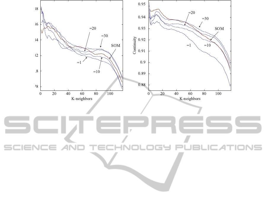
Figure 2: Trustworthiness (a) and continuity (b) as a function of k-neighbors.

hand, when the interaction parameter α is one, the er-

ror is 0.075. Then, the error is gradually increased to

0.126 when the parameter is 50. The topographic er-

ror is 0.496 when the parameter is one, which is much

larger than 0.009 by the conventional SOM. However,

when the parameter is 10, the error becomes 0.051. In

addition, when the parameter is 20 and 40, the errors

are completely zero. Training errors are the lowest

(0.068) when the parameter is one. When the param-

eter is increased, the error becomes larger. The gen-

eralization error is the lowest when the parameter is

ten and the largest when the parameter is 20. Com-

pared with errors (0.205) by the conventional SOM,

all errors by the interaction are much smaller.

Figure 2(a) shows trustworthiness as a function of

k-neighbor. As can be seen in the ﬁgure, the trust-

worthiness is the lowest over almost all neighbors

when the parameter is one. As the parameter is in-

creased from 10 to 20, the trustworthiness is gradu-

ally increased. Then, when the k-neighbor is 30, the

trustworthiness is higher than that by the conventional

SOM in red. Figure 2(b) shows the continuity as a

function of k-neighbor. When the parameter is one,

the continuity is the lowest and far from the level by

the conventional SOM. As the parameter is increased,

the continuity is increased over almost all range of k-

neighbor. When the k-neighbor is 30, the continuity

is larger for the majority of k-neighbors.

Figure 3 shows U-matrices by the conventional

SOM (a) and interaction (b)-(f). When the parame-

ter is one in Figure 3(b), boundaries to be represented

in warmer colors seem to be scattered over the matrix.

When the parameter is increased to ten in Figure 3(c),

the boundaries in warmer colors are located on the

both sides. When the parameter is increased further

to twenty in Figure 3(d), the two explicit boundaries

in warmer colors can be seen on the lower side of the

map, which are very close to those obtained by the

conventional SOM in Figure 3(a). When the param-

eter is further increased to thirty and forty in Figure

3(e) and (f), the two boundaries seem to be more ex-

plicit than those by the conventional SOM in Figure

3(a).

4 CONCLUSIONS

In this paper, we have proposed a new type of

information-theoretical model in which the individ-

uality and collectiveness of neurons are controlled

by the interaction parameter α. As the interaction

parameter α is increased, the effect of collective-

ness becomes larger. We have applied the method to

the production of the self-organizing maps with the

ionosphere data from the machine learning database.

Experimental results conﬁrmed that improved per-

formance could be observed in terms of all mea-

sures, namely, quantization, topographical, training

and generalization errors by controlling the interac-

tion parameter α. In addition, the trustworthiness and

continuity over almost all ranges of k-neighbors be-

come gradually larger as the interaction parameter α

is larger. This means that the collectiveness can be

used for neurons to cooperate with others like SOM.

Finally, the feature maps obtained by our method

showed sharper class boundaries compared with those

by the conventional SOM.

The present experimental results are only prelim-

inary ones with an initial condition. Thus, we need

to compare the results more rigorously. However, we

can at least shows a possibility that the ﬂexible inter-

action of ITN and CTN can be used to produce im-

proved performance and explicit class structure.

NCTA 2011 - International Conference on Neural Computation Theory and Applications

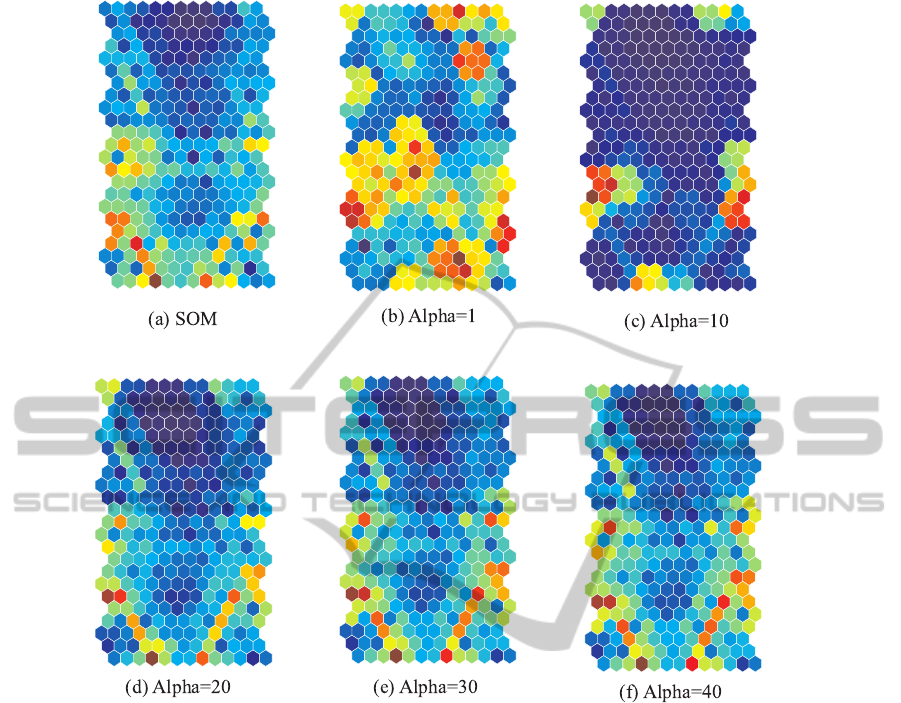
Figure 3: U-matrices by the conventional SOM (a), and interaction when the interaction parameter is changed from one (a) to

40 (f).

REFERENCES

Bauer, H.-U. and Pawelzik, K. (1992). Quantifying the

neighborhood preservation of self-organizing maps.

IEEE Transactions on Neural Networks, 3(4):570–

578.

Bishop, C. M. (1995). Neural networks for pattern recog-

nition. Oxford University Press.

Costa, J. A. F. Clustering and visualizing som results. In

Fyfe et al., C., editor, Proceedings of IDEAL2010, vol-

ume LNCS6283, pages 334–343. Springer.

Demartines, P. and Herault, J. (1997). Curvilinear com-

ponent analysis: a self-organizing neural network for

nonlinear mapping of data sets. IEEE Transactions on

Neural Networks, 8(1).

Georg Polzlbauer, M. D. and Rauber, A. (2006). Ad-

vanced visualization of self-organizing maps with

vector ﬁelds. Neural Networks, 19:911–922.

Joshua B. Tenenbaum, V. d. S. and Langford, J. C. (2000).

A global framework for nonlinear dimensionality re-

duction. SCIENCE, 290:2319–2323.

Kamimura, R. (2003). Information-theoretic competitive

learning with inverse Euclidean distance output units.

Neural Processing Letters, 18:163–184.

Kamimura, R., Kamimura, T., and Shultz, T. R. (2001a). In-

formation theoretic competitive learning and linguis-

tic rule acquisition. Transactions of the Japanese So-

ciety for Artiﬁcial Intelligence, 16(2):287–298.

Kamimura, R., Kamimura, T., and Uchida, O. (2001b).

Flexible feature discovery and structural information

control. Connection Science, 13(4):323–347.

Kaski, S., Nikkila, J., Oja, M., Venna, J., Toronen, P., and

Castren, E. (2003). Trustworthiness and metrics in

visualizing similarity of gene expression. BMC Bioin-

formatics, 4(48).

Kiviluoto, K. (1996). Topology preservation in self-

organizing maps. In In Proceedings of the IEEE Inter-

national Conference on Neural Networks, pages 294–

299.

Kohonen, T. (1988). Self-Organization and Associative

Memory. Springer-Verlag, New York.

Kohonen, T. (1995). Self-Organizing Maps. Springer-

Verlag.

INDIVIDUALLY AND COLLECTIVELY TREATED NEURONS AND ITS APPLICATION TO SOM

Lee, J. A. and Verleysen, M. (2008). Quality assessment

of nonlinear dimensionality reduction based on K-ary

neighborhoods. In JMLR: Workshop and conference

proceedings, volume 4, pages 21–35.

Polzlbauer, G. (2004). Survey and comparison of quality

measures for self-organizing maps. In Proceedings of

the ﬁfth workshop on Data Analysis (WDA04), pages

67–82.

Rose, K., Gurewitz, E., and Fox, G. C. (1990). Statistical

mechanics and phase transition in clustering. Physical

review letters, 65(8):945–948.

Roweis, S. T. and Saul, L. K. (2000). Nonlinear dimen-

sionality reduction by locally linear embedding. SCI-

ENCE, 290:2323–2326.

Sammon, J. W. (1969). A nonlinear mapping for data struc-

ture analysis. IEEE Transactions on Computers, C-

18(5):401–409.

Tasdemir, K. and Merenyi, E. (2009). Exploiting data topol-

ogy in visualization and clustering of self-organizing

maps. IEEE Transactions on Neural Networks ,

20(4):549–562.

Ultsch, A. (2003a). Maps for the visualization of high-

dimensional data spaces. In Proceedings of the 4th

Workshop on Self-organizing maps, pages 225–230.

Ultsch, A. (2003b). U*-matrix: a tool to visualize clusters in

high dimensional data. Technical Report 36, Depart-

ment of Computer Science, University of Marburg.

Venna, J. (2007). Dimensionality reduction for visual explo-

ration of similarity structures. Dissertation, Helsinki

University of Technology.

Venna, J. and Kaski, S. (2001). Neighborhood preserva-

tion in nonlinear projection methods: an experimental

study. In Lecture Notes in Computer Science, volume

2130, pages 485–491.

Vesanto, J. (1999). SOM-based data visualization methods.

Intelligent-Data-Analysis, 3:111–26.

Vesanto, J., Himberg, J., Alhoniemi, E., and Parhankan-

gas, J. (2000). SOM toolbox for Matlab. Technical

report, Laboratory of Computer and Information Sci-

ence, Helsinki University of Technology.

Villmann, T., Herrmann, R. D. M., and Martinez, T.

(1997). Topology preservation in self-organizing fea-

ture maps: exact deﬁnition and measurment. IEEE

Transactions on Neural Networks, 8(2):256–266.

NCTA 2011 - International Conference on Neural Computation Theory and Applications