DESIGN OF RECURRENT FUZZY NEURAL NETWORK AND
GENERAL REGRESSION NEURAL NETWORK CONTROLLER
FOR TRAVELING-WAVE ULTRASONIC MOTOR
Tien-Chi Chen
1
, Tsai-Jiun Ren
2
and Yi-Wei Lou
1
1
Department of Electrical Engineering, Kun Shan University, Tainan, Taiwan
2
Department of Information Engineering, Kun Shan University, Tainan, Taiwan
Keywords: Traveling-wave ultrasonic motor, TWUSM, Recurrent fuzzy neural network, RFNN, Back-propagation
algorithm, Lyapunov theorem, General regression neural network, GRNN, Dead-zone.
Abstract: The traveling-wave ultrasonic motor (TWUSM) has significant features such as high holding torque at low
speed range, high precision, fast dynamics, simple structure, no electromagnetic interference. The TWUSM
has been used in many practical areas such as industrial, medical, robotic, and automotive applications.
However, the dynamic model of the TWUSM motor has the nonlinear characteristic and dead-zone problem
which varies with many driving conditions. This paper presents a novel control scheme, recurrent fuzzy
neural network (RFNN) and general regression neural network (GRNN) controller, for a TWUSM control.
The RFNN provides a real-time control such that the TWUSM output can track the reference command. The
back-propagation algorithm is applied in the RFNN to automatically adjust the parameters on-line. The
adaptive laws of the RFNN are derived by Lyapunov theorem such that the stability of the system can be
absolute. The GRNN controller is appended to the RFNN controller to compensate the dead-zone of the
TWUSM system using a predefined set. The experimental results are provided to demonstrate the
effectiveness of the proposed controller.
1 INTRODUCTION
In recent years, the TWUSM is a new type motor,
which is driven by the ultrasonic vibration force of
piezoelectric elements. It has an excellent
performance and many useful features (Sashida and
Kenjo, 1993), such as high torque at low speed,
quiet operation, light weight and compact in size,
quick response, wide velocity range, high efficiency,
simple structure, easy production process, no
electro-magnetic interference and so on (Ueha and
Tomikawa, 1993); (Uchino, 1997). Therefore, the
TWUSM can be used in many regions like
industrial, medical, automotive applications,
aerospace science, and accurate positioning
actuators (Huafeng eu al., 2005).
The TWUSM is a new type of actuator which is
different to the conventional electromagnetic
motors, for instance, the control technique and the
operating principles. Since the TWUSM composed
of piezoelectric ceramics instead of electromagnetic
windings in motor structures (Uchino, 1998), the
driving principles of the TWUSM are based on the
ultrasonic vibration of piezoelectric elements and
mechanical frictional force (Chen et al., 2008).
However, the dynamic model of the TWUSM
motor is very complicated and has the nonlinear
characteristic, which varies with many driving
conditions. The TWUSM parameters are nonlinear
and time varying due to the temperature increasing
and different motor drive operating conditions, such
as driving frequency, source voltage, and load torque
(Sashida and Kenjo, 1993). Moreover, the control
characteristics of the TWUSM are very complex to
analyze and modeling accurately (Hagood and
Mcfarland, 1995).
In general, the traveling-wave ultrasonic motor
drive and digital control system may apply three
independent control methods which are drive
frequency control, supplied voltage control and
phase difference control of applied voltage. In phase
difference control method, the motor shows a
variable dead-zone in the control input (phase
difference of applied voltages) against with
operating frequency. By the way, dead-zone will due
to a large static friction torque appears at low speed.
31
Chen T., Ren T. and Lou Y..
DESIGN OF RECURRENT FUZZY NEURAL NETWORK AND GENERAL REGRESSION NEURAL NETWORK CONTROLLER FOR TRAVELING-
WAVE ULTRASONIC MOTOR.
DOI: 10.5220/0003677800310040
In Proceedings of the International Conference on Neural Computation Theory and Applications (NCTA-2011), pages 31-40
ISBN: 978-989-8425-84-3
Copyright
c
 2011 SCITEPRESS (Science and Technology Publications, Lda.)

Hence, it is difficult to design a perfect angle
controller which can accurate control at all times.
According to practical control issues, there have
been reported many speed controllers based on PI
(proportional plus integral) controller uses
mathematical model of the motor.
Because the control algorithms of the PI
controller are simple, and the controllers have the
advantages such as high-stability margin and high-
reliability when the controllers are tuned properly,
the PI controller can use to drive the common
motors. However, the PI controller can not maintain
these virtues at all times. Especially, the ultrasonic
motor has the nonlinear speed characteristics which
vary with drive operating conditions. In order to
overcome these difficulties, the dynamic controller
with adjustable parameters and online learning
algorithms will be suggested for the unknown or
uncertain dynamics systems (Bal and Bekiroglu,
2004); (Bal and Bekiroglu, 2005).
In the past few years, there has been much
research on the applications of neural networks
(NNs) in order to deal with the nonlinearities and
uncertainties in control systems (Alessandri et al.,
2007); (Liu, 2007); (Abiyev and Kaynak, 2008).
According to the structures of the NNs, the NNs can
be mainly classified as feedforward NNs and
recurrent NNs (RNNs) (Lin and Hsu, 2005). It is
well known that feedforward NNs is capable of
approximating any continuous functions closely. But
the feedforward NNs are a static mapping without
the aid of delays. The feedforward NNs is unable to
represent a dynamic mapping. Although, the
feedforward NNs presented in much research has
used to deal with delay and dynamical problems.
The feedforward NNs must require a large number
of neurons to express dynamical responses (Ku and
Lee, 1995). Furthermore, the calculations of the
weights do not update quickly and the function
approximation is sensitive to the training data.
On the other hand, RNNs (Juang et al., 2009)
have superior capabilities compared with
feedforward NNs, such as dynamics response and
the information-storing ability for later use. Since
the recurrent neuron has an internal feedback loop, it
captures the dynamic response of a system without
external feedback through long delays. Thus, the
RNNs are a dynamic mapping and displays good
control performance in the presence of the
unknowable and time-varying model dynamics
(Stavrakouds and Theochairs, 2007). As the result
which is exhibited previously, the RNNs are better
suited for dynamical systems than the feedforward
NNs.
Furthermore, if the number of the hidden neurons
is chosen too many, the computation loading is
heavy so that it is not suitable for online practical
applications. If the number of the hidden neurons is
chosen too less, the learning performance may not
be good enough to achieve the desired control
performance. To solve this problem, this scheme
proposed a novel controller, recurrent fuzzy neural
networks (RFNN), for maintain high accuracy.
The RFNN control has a number of attractive
advantages compared to the RNN control. For
example, superior modeling performance due to
local modeling and the fuzzy partition of the input
space, linguistic description in terms of dynamic
fuzzy rules, proper structure learning based on
training examples, and parsimonious models with
smaller parametric complexity (Lin and Chen,
2005). Thus, RFNN systems which combine the
capability of fuzzy reasoning to handle uncertain
information and the capability of artificial recurrent
neural networks to learn processes, is used to deal
with nonlinearities and uncertainties of the
TWUSM.
In spite of the perfect RFNN controller has
designed, there still exists a challenge for
considering the TWUSM as a plant. In the proposed
RFNN control schemes, the controller is effective in
handling the small characteristics variations of the
motor due to the updating of the connecting weights
in the RFNN. However, the RFNN controller is not
able to fully compensate for the dead-zone effect,
and therefore the dynamic response is deteriorated
(Senjyu et al., 2002). For the reason, an angle
control scheme for the TWUSM with the dead-zone
compensation based on RFNN is presented in this
scheme. The general regression neural networks
(GRNN) is adopted to determine the dead-zone
compensating input and decouple the output of the
RFNN. Because of the saturation reverse effect,
phase difference control is not adequate for a precise
angle control. Therefore the drive frequency has to
be implemented in addition, which leads to a more
accurate control strategy. Thus, the GRNN based on
RFNN control scheme which apply both the driving
frequency and phase difference constructing as the
dual-mode control method was presented. The
proposed controller can take the nonlinearity into
account and compensate the dead-zone of TWUSM.
Further, this also provides the robust performance
against the parameter variations. The usefulness and
validity of the proposed control scheme is examined
through experimental results. The experimental
results reveal that the GRNN base on the RFNN
controller maintains stable and good performance on
NCTA 2011 - International Conference on Neural Computation Theory and Applications
32

different motion conditions. These demonstrate the
reliability of the proposed control scheme and
effectiveness of the MGRNN modeling control
scheme in this scheme.
2 THE CONTROL SCHEME
The nonlinear dynamic system of the TWUSM is
expressed as:
() ()() ()
f
gutdt   

(1)
where
()
f

and
()
g

are unknown functions, and
assume they are bounded. u(t) is the control input,
d(t) is the external disturbance, and

is rotor angle
displace of the TWUSM.
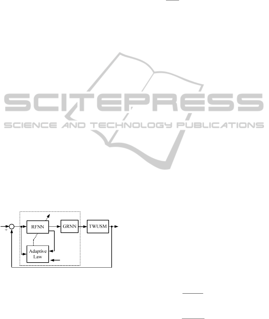
The proposed control scheme, illustrated as the
Figure 1, is composes of two main blocks, RFNN
and GRNN controller. The RFNN provides a real-
time control such that the TWUSM output can track
the reference command
r

. The back-propagation
algorithm is applied in the RFNN to automatically
adjust the parameters on-line. The adaptive laws of
the RFNN are derived by Lyapunov Theorem such
that the stability of the system can be absolute.

,
T
m

,
T


,
T
r

are the training parameters of adaptive
update law, and
1

,
2

,
3

,
4

,
5

are the learning
rates. The GRNN controller is appended to the
RFNN controller to compensate the dead-zone of the
TWUSM system using a predefined set. The GRNN
controller is designed to avoid the dead-zone
response of the TWUSM.
,,,,wm r







G
u
123
45
,,,
,



E

R
EFF
u
r

, ,
,
T
m
TT
r





Figure 1: The control structure.
2.1 Recurrent Fuzzy Neural Networks
Control System
To design a controller such that the TWUSM output
can track the reference command. First, define the
tracking error vector as


,
T
Eee

(2)
where
r
e




is the angle tracking error. From (1)
and (2), an ideal controller can be chosen as
*
1
() [ ( ) () ]
()
T
rn n
n
ut f dt KE
g




(3)
where


21
,
T
K
kk
,
1
k
and
2
k
are positive
constants. Applying (2) to (3), the error dynamics
can be expressed as
12
0ekeke


 
(4)
If K is chosen to correspond to the coefficients of a
Hurwitz polynomial, that is a polynomial whose
roots lie strictly in the open left half of the complex
plane, then the result achieved where


lim 0
t
et


for any initial conditions. Nevertheless, the functions
()
f

and
()
g

aren’t accurate known and the
external load disturbances is perturbed. Thus, the
ideal controller


*
ut
cannot be practical
implemented. Therefore, the RFNN system will be
designed to approximate this ideal controller.
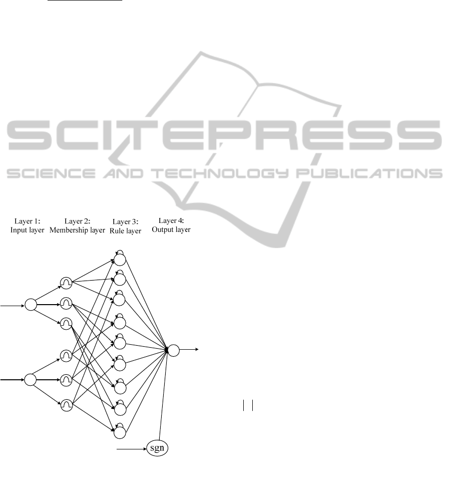
Figure 2 shows the four-layer RFNN structure of
the angle controller, which is comprised by the input
layer, membership layer, rule layer, and output layer.
The superscript of symbol y means the ordinal
number of the layer, and the subscript of symbol y
means its number. The symbol
w expresses the
weight of the signals. The model of RFNN is
summarized as follows:
(1) Input Layer. The inputs of the RFNNr are
1
e
x
e

and
1
e
x
e



. The outputs of input layer are
1
,
ei
y
and
1
,
ei
y

, which are equal to the inputs:
11
,
; 1~3
ei e
yxi
(5)
11
,
; 1~3
ei e
yxi

(6)
(2) Membership Layer. There are three
membership functions for e, and
e

, respectively.
The three signals are sent to calculate the degree
belonging to the specified fuzzy set. The outputs
2
,ei
y
and
2
,ei
y

are as follows.
2
1
,,
2
,
,
exp ; 1 ~ 3
ei ei
ei
ei
ym
yi





 





(7)
2
1
,,
2
,
,
exp ; 1 ~ 3
ej ej
ej
ej
ym
yi





 








(8)
where m and

are the mean and the standard
deviation of the Gaussian function. They express the
DESIGN OF RECURRENT FUZZY NEURAL NETWORK AND GENERAL REGRESSION NEURAL NETWORK
CONTROLLER FOR TRAVELING-WAVE ULTRASONIC MOTOR
33

different membership functions of the RFNN, so the
output of the layer can represents the belonging
degree of the input to the fuzzy rule.
(3) Rule Layer. The outputs
3
k
y
of the rule layer can
be expressed as
3
322
,,
10 ( 1)
1
() (1 ) () ()
1 100 exp
D
kk
keiej
ry t
y
tytyt




(9)
where
3( 1)kij  
,
1~3,i  1~3j 
and
1~9k

.
D
k
r
are the weights. The value of
3
k
y
is always
positive and between zero and two.
(4) Output Layer. The output
4
o
y
of the RFNN can
be expressed as
9
43T
1
T
ˆ
+ sgn(E PB)
ˆ
( , , , )+ sgn(E PB)
RFNN o k k
k
T
uywy
wxmr






(10)
where
33 3
12 9
(, , ,)
T
x
mr yy y 




fuzzy rule
function vector, and


12 9
T
www w 
adjustable output weight vector,

a small positive
constant, and


,
T
E
ee

.
k
w
D
k
r
1
e
x
1
e
x

1
,1e
y
3
k
y
4
o
y







R
FNN
u



e
e

1
,2e
y
1
,3e
y
1
,1e
y

1
,2e
y

1
,3e
y

2
,1e
y
2
,2e
y
2
,3e
y
2
,1e
y

2
,2e
y

2
,3e
y

3
k
I
ˆ

P
B
T
E
Figure 2: The structure of Recurrent Fuzzy Neural
Networks.
Assume there exists an optimal RFNN to
approximate the ideal control law such that
** **** **
(, , , , )
T
RFNN
uu ewm r w

 
(11)
where

is a minimum reconstructed error,
*
w
,
*
m
,
*

,
*
r
and
*

are optimal parameters of w , m ,

,
r and

, respectively. Thus, the RFNN control law
is assumed to take the following form:
T
ˆ
ˆ
ˆ
+ sgn(E PB)
T
RFNN
uu w  
(12)
where
ˆ
w
,
ˆ
m
,
ˆ

,
ˆ
r
and
ˆ

are estimations of the
optimal parameters, provided by tuning algorithms
to be introduced later. Subtracting (12) from (11), an
approximation error
u

is obtained as
*** T
*T
ˆ
ˆ
ˆ
sgn(E PB)
ˆ
ˆ
sgn(E PB)
T
T
TT
uu uw w
ww


 




(13)
where
*
ˆ
ww w



and
*
ˆ

 

. The linearization
technique transforms the multidimensional
receptive-field basis functions into a partially linear
form such that the expansion of


in Taylor series
becomes
33
19
T
mrv
yy m rO







 

(14)
where
33*3
ˆ
kk k
yy y



,
3*
k
y
the optimal parameter of
3
ˆ
k
y
,
3
ˆ
k
y
the estimated parameter of
3*
k
y
,
*
ˆ
mm m

,
*
ˆ





,
*
ˆ
rr r



,
v
O
higher-order terms,
33
ˆ
19
/ ... / |
T
mmm
ym ym


 

,
33
ˆ
19
/.../ |
T
yy





 

and
33
ˆ
19
/... / |
T
rrr
yr yr


 

.
Equation (14) can be rewritten as
*
ˆ
mrv
mrO



   

(15)
Substituting (15) into (13), it can be rewritten as:
T
T
ˆ
()
ˆ
ˆ
()sgn(EPB)
ˆ
ˆ
ˆ
= ( ) sgn(E PB)
T
mrv
T
mrv
TT
mr
uw m rO
wm rO
wwm r D






    


 
   


(16)
where
*
()
T
T
mrv
Dw m r wO




 

is the
uncertainty term, and this term is assumed to be
bounded with a small positive constant

（
let D


） . From (1), (4) and (16), an error
equation is obtained
*
T
()
ˆ
ˆ
ˆ
( ) sgn(E PB)
TT
mr
E AE B u u AE Bu
A
EBw w m r D


 
  







(17)
Consider the RFNN dynamic system represented by
(1), if the RFNN control law is designed as (12) with
the adaptation laws for networks parameters shown
in (18)–(22), the stability of the proposed RFNN
control system can be guaranteed. where
1

,
2

,
3

,
4

and
5

are strictly positive constants.
NCTA 2011 - International Conference on Neural Computation Theory and Applications
34

1
ˆ
ˆ
T
wEPB  

(18)
2
ˆ
ˆ
TT
m
mwEPB  

(19)
3
ˆ
ˆ
TT
wE PB

 

(20)
4
ˆˆ
TT
r
rwEPB  

(21)
5
ˆ
T
E
PB  

(22)
Proof:
Define a Lyapunov function candidate as
12
2
345
11 1
() ( )
22 2
111
222
TTT
TT
Vt EPE trww mm
rr

 

 

 

 
(23)
where P is a symmetric positive definite matrix
which satisfies the following Lyapunov equation
T
A
PPA Q
(24)
where Q is a positive definite matrix. Here, the
estimation error of the uncertainty bound is defined
as
ˆ

 

. Taking the differential of the
Lyapunov function (23) and using (16) and (24), it is
concluded that

12 3 45
1
ˆ
ˆ
()
2
11 1 11
ˆ
ˆˆ
ˆˆ
TTTT
C
TTTT
Vt EQE EPBw w m r u D
mr
ww mm rr


 
 

       


 



  


(25)
Take (18)-(22) into (25), the derivative of V can be
rewritten as

5
11
ˆˆ
()
2
1
( ) 0
2
TT T
C
TT
V t E QE E PBD E PBu
EQE EPB D




    
   


(26)
Therefore no matter what the situation is, the
derivative of V respect to time is smaller than zero.
Since


0Vt

is negative semi-definite (i.e.,




0Vt V

), which implies E,
w

,
m

,


,


and
r

are bounded. Let function




/2
T
F
tEQE Vt

,
and integrate function with respect to time.
Because V(0) is bounded, and V(t) is bounded,
the following result is obtained:

0
lim
t
t
Fd 



(27)
Also, since


F
t

is bounded, so by Barbalat’s
Lemma, it can be shown that

lim 0
t
Ft


. It implies
that


E
t
will converge to zero as
t 
. As a
result, the stability of the proposed control system
can be guaranteed.
2.2 Convergence Analysis of RFNN
Although the stability of the adaptive RFNN control
system can be guaranteed, the parameters
ˆ
w
,
ˆ
m
,
ˆ

and
ˆ
r
in (18)–(21) can not be guaranteed within a
bound value. The output of the RFNN is bounded,
whether the means, the standard deviation of the
Gaussian function and weights are bounded. Define
the constrain sets
w
,
m
,

and
r
respectively


ˆ
w
Uww
(28)


ˆ
m
Umm
(29)


ˆ
U


 
(30)


ˆ
r
Urr


(31)
where

is a two-norm of vector,
w
,
m
,

and
r
are positive constants, and the adaptive laws (18)-
(21) can be modified as follows


1
11
2
ˆˆ
ˆˆ ˆ
, if 0
ˆ
ˆˆ
ˆˆ ˆ
ˆˆ
, if 0
ˆ
T TT
T
TT TT
EPB w wor w wandEPBw
w
ww
E PB E PB w w and E PBw
w








  




(32)

2
22
2
ˆˆ
ˆˆˆ
, if 0
ˆ
ˆˆ
ˆˆ ˆ ˆˆ
, if 0
ˆ
TT TT
m m
T
TT TT T T
mm m
wE PB m m or m m and E PBw m
m
mm
wE PB wE PB m m and E PBw m
m








  




(33)


3
33
2
ˆˆˆˆˆ
, if 0
ˆ
ˆ
ˆ
ˆˆ
ˆˆˆ
, if 0
ˆ
TT TT
T
TT TT T T
wE PB or and E PBw
wE PB wE PB and E PBw
 
 



  







  




(34)


4
44
2
ˆ
ˆˆ ˆˆ
, if 0
ˆ
ˆ
ˆ
ˆ
ˆˆˆˆ
, if 0
ˆ
TT TT
r r
T
TT TT T T
rr r
wE PB r r or r r and E PBw r
r
rr
wE PB wE PB r r and E PBw r
r








  




(35)
If the initial values
ˆ
(0)
w
wU

,
ˆ
(0)
m
mU
,
ˆ
(0) U



and
ˆ
(0)
r
rU

then the adaptive laws (32)-
(35)guarantee that
ˆ
()
w
wt U

,
ˆ
()
m
mt U
,
ˆ
()
tU



and
ˆ
()
r
rt U

for all
0t 
.
Define a Lyapunov function as
1
ˆ
ˆ
2
T
w
vww
(36)
And, the derivative of the Lyapunov function is
presented as
ˆ
ˆ
T
w
vww


(37)
Assume the first line of (32) is true, either
ˆ
ww

or


ˆ
ˆ
ˆ
0
TT
w w and E PBw


. Substituting the first
line of (32) into (37), which becomes
1
ˆ
ˆ
0
TT
w
vEPBw 



. As a result,
ˆ
ww

is
guaranteed. In addition, when
ˆ
ˆ
ˆ
0
TT
w w and E PBw


,
DESIGN OF RECURRENT FUZZY NEURAL NETWORK AND GENERAL REGRESSION NEURAL NETWORK
CONTROLLER FOR TRAVELING-WAVE ULTRASONIC MOTOR
35

11
2
ˆ
ˆ
ˆˆ
ˆ
ˆ
0
ˆ
T
TT T T
w
ww
vEPBw EPBw
w
  

. That
ˆ
ww

can be also assured. Thereby, the initial
value of
ˆ
w
is bounded,
ˆ
w
is bounded by the
constraint set
w
for
0t 
. Similarly, it can be
proved that
ˆ
m
is bounded by the constraint set
m
,
ˆ

is bounded by the constraint set

and
ˆ
r
is
bounded by the constraint set
r
for
0t 
.
When the condition
ˆ
ww
or

ˆ
ˆˆ
0
TT
w w and E PBw
,
ˆ
mm
or


ˆ
ˆˆ
0
TT
m
m m and E PBw m
,
ˆ



or


ˆˆˆ
0
TT
and E PBw

  
,
ˆ
rr

or


ˆ
ˆ
ˆ
0
TT
r
r r and E PBw r
, the stability analysis
the same as (33), (34) and (35). In the other
situation, the condition
ˆ
ww
and
ˆ
ˆ
0
TT
E PBw


,
ˆ
mm
and
ˆˆ
0
TT
m
EPBw m


,
ˆ

 
and
ˆ
ˆ
0
TT
E PBw

 
,
ˆ
rr
and
ˆ
ˆ
0
TT
r
E PBw r
is
occurred, the Lyapunov function can be rewritten as
follows



1
2345
22
2
11
ˆ
ˆˆˆ ˆ
)
2
1111
ˆ
ˆˆˆ
ˆˆ
1
ˆ
ˆˆˆ
()
2
ˆˆ
ˆ
ˆˆ ˆ
( ) (
ˆ
TTTT T T T
w C
TTT
TT
TT T TTTT
Cm
T
TTT T
r
vEQEEPBwwmw wrDuww
mr
mm rr
ww mm
EQE EPBD u EPB w w EPBm
wm
wEPB w




 




      

     
 








2
5
ˆ
1
ˆ
ˆ
)
ˆ
T
TT
rr
E PBr
r





(38)
Equation


2
22
*
ˆˆ
/2 0
T
ww w w w 

, which is
according to
*
ˆ
ˆ
www
. Similarly,
*
ˆˆ
mmm
,
*
ˆˆ

 
and
*
ˆˆ
rrr
can
be proved. Finally, it is obtained as




22
22
5
2
22
*
2
2
22
*
2
ˆ
ˆ
1
ˆ
ˆˆ
ˆ
2
ˆ
ˆ
ˆ
ˆ
1
ˆ
ˆ
ˆ
ˆˆ
ˆ
ˆ
ˆ
1
ˆ
ˆ
2
ˆ
ˆ
1
ˆˆ
( )
2
ˆ
1
(
2
TT
TT T T TTT
wCm
TT
TT TT
r
TT T
TTT
m
ww mm
v EQE EPBD EPBu EPB w wEPBm
wm
rr
wE PB wE PBr
r
www
EQE EPB w
w
mmm
w E PBm
m





    
  

  














2
22
*
2
2
22
*
2
ˆ
ˆˆ
)
ˆ
ˆ
1
ˆˆ
( )
2
ˆ
1
0
2
TTT
TTT
r
T
wEPB
rrr
wEPBr
r
EQE







 


(39)
Using the same discussion shown in previous
section, the stability property can be also guaranteed
since
0E 
as
0t 
.
2.3 General Regression Neural
Networks Control System Design
As a common nonlinear problem, dead-zone often
appears in the control system, which not only makes
steady-sate error, but also deteriorates the dynamic
quality of the control systems. As for the dead-zone
compensation problems, general regression neural
networks (GRNN) control methods is proposed to
solve this problems. The GRNN is a powerful
regression tool with a dynamic network structure
and training speed is extremely fast. Due to the
simplicity of the network structure and ease of
implementation, it can be widely applied to a variety
of fields.
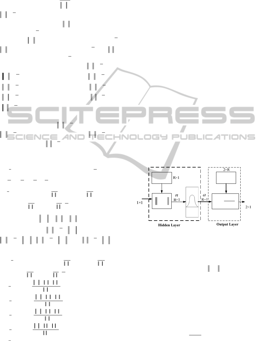
The GRNN scheme which shows in Figure 3 is
suggested for the nonlinear compensation of the
system input. Where the input u is the output of the
RFNN,
1
G
W
is the weight of the hidden layer,
2
G
W
is
the weight of the output layer, a is the output of the
hidden layer,
G
u
is the output of the output layer.
2
G
G
Wa
u
a



G
u
dist
u
2
G
W
1
G
W
Figure 3: The structure of the GRNN.
The GRNN is composed of two layers, which are
the hidden layer and the output layer. The input
u
of the GRNN means a torque which calculated by
the RFNN. The outcome n of
dist
is represented
the Euclidean distance between input u and each
elements of
1
G
W
. Then n pass by a Gaussian function.
When the Euclidean distance between u and
1
G
W
is
far, the element of the output a is approach to zero.
In the other hand, the Euclidean distance is short and
the element of the output a is approach to one. The
Gaussian function is
2
exp
nm
a










(40)
NCTA 2011 - International Conference on Neural Computation Theory and Applications
36

Where
m
and

are the center and the stand
deviation of the Gaussian function respectively. In
order to increase the discrimination and have a better
performance, the stand deviation

value of the
Gaussian function is chose low.
The relation function of output layer can be
expressed as
2
G
G
Wa
u
a



(41)
The output vector of hidden layer a is multiplied
with appropriate weights
2
G
W
to sum up for produce
the output
G
u
of the GRNN. The output
G
u
composed of frequency control
f
u
and phase control
P
u
is expressed as
T
Gfp
uuu



(42)
Applying the GRNN controller, the dead-zone of the
TWUSM will be compensated as desired.
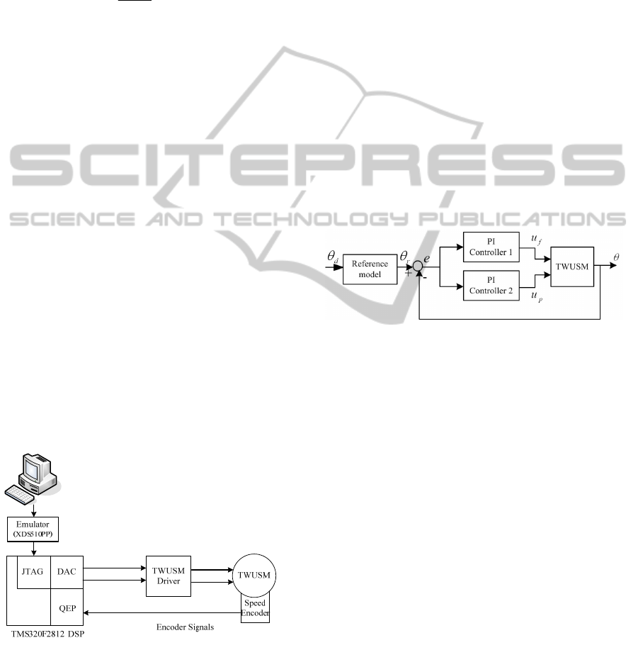
3 EXPERIMENTS
To prove the feasibility of the scheme, the
experiments are required. The structure of the
experiment includes DSP program and hardware
driving circuit. It is shown in the Figure 4. The
TMS320F2812 DSP experiment board is applied as
the computing core. The DSP program was coded by
C language. After compile, assemble and link, the
executing file will be generated by c2000 code
composer (CCS), additionally the executing file was
be executed in the same windows interface.
sin
m
Vt

sin( )
m
Vt

 
Frequency-Controlled
Voltage ( )
f
u
Phase-Controlled
Voltage ( )
P
u
Figure 4: Experimental system of the TWUSM.
In the experiments, there are three different
controllers chosen for comparison.
(i) The proposed control scheme, RFNN and
GRNN controller.
(ii) The RFNN only, without GRNN controller.
The control algorithm of RFNN only is the same as
RFNN of the proposed control scheme.
(iii) The PI controller. The PI controller is the one
of the most used controller in linear system. The
control PI controller has important advantages such
as simple structure and easy to design. Therefore, PI
controllers are used widely in industrial application.
Owing to the absence of the mathematical model of
the TWUSM, the PI controller parameters are
chosen by trial and error in such a way that the
optimal the performance occurs at rated conditions.
The block diagram of the angle control system for
ultrasonic motor by PI controller shown in Figure 5.
Where
r

and

are command and rotor angle, e(k)
is the tracking error,
f
u
is the frequency command,
p
u
is the phase different command, respectively.
The parameters of the PI controller are selected as
1000
P
K

and
100
I
K

. The parameters of the PI
controller 2 are selected as
1000
P
K 
and
100
I
K

.
Figure 5: The block diagram of the dual-mode PI control.
Figures 6 to 8 show the experimental results of
the proposed control scheme, the RFNN only, and
the PI control respectively, for a periodic square
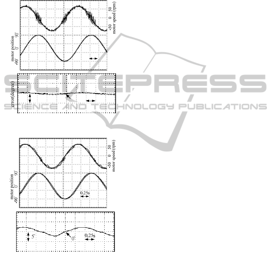
angle command from -90 to 90 degree. Figures 9 to
11 show the experimental results of the proposed
control scheme, the RFNN only, and the PI control
respectively, for a sinusoidal angle command from -
90 to 90 degree. In each Figure (a) shows the
TWUSM angle response and speed response. In
each Figure (b) shows the angle error between angle
command and angle response.
Observing the experimental results of the
proposed control scheme in Figures 6 and 9, the
tracking errors both can converge to an acceptable
region and the control performance is excellent. The
proposed controller retains control performance and
has not any dead-zone in the constructed.
The experimental results of the RFNN only in
Figures 7 and 10 show that the tracking error is
similar to the proposed control scheme. However,
the drawbacks of the RFNN controller are interfered
with the dead-zone and the motor speed has the
serious chattering phenomenon in slow speed nearby
zero.
DESIGN OF RECURRENT FUZZY NEURAL NETWORK AND GENERAL REGRESSION NEURAL NETWORK
CONTROLLER FOR TRAVELING-WAVE ULTRASONIC MOTOR
37

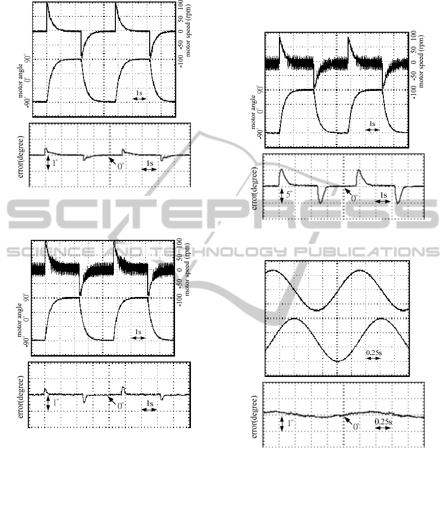
(a)
(b)
Figure 6: The experimental result of the proposed control
scheme for a periodic angle square command from -90 to
90 degree.
(a)
(b)
Figure 7: The experimental result of the RFNN only for a
periodic square angle command from -90 to 90 degree.
In Figures 8 and 11 illustrated that the PI
controller has a chattering phenomenon like the
RFNN only and larger tracking error.
4 CONCLUSIONS
The proposed control scheme, RFNN and GRNN
controller, has been applied to the TWUSM in the
paper. Many concepts such as controller design and
the stability analysis of the controller are introduced.
Furthermore, experiment results are shown and
proven that the proposed control scheme is feasible
and the performance of the proposed method is
better than the others.
(a)
(b)
Figure 8: The experimental result of the PI control for a
periodic square angle command from -90 to 90 degree.
(a)
mo
t
o
r
posi
t
ion
-90° 0° 90°
motor speed (rpm)
-50 0 50
(b)
Figure 9: The experimental result of the proposed control
scheme for a sinusoidal angle command from -90 to 90
degree.
The proposed control scheme includes the RFNN
controller and the GRNN controller. The RFNN
controller is designed to track the reference angle.
The variables of membership function and weights
can be updated by the adaptive algorithms.
Moreover, all parameters of the proposed RFNN
controller are tuned in the Lyapunov sense; thus, the
stability of the system can be guaranteed. In the
RFNN, a compensated controller is designed to
recover the residual part of approximation error. The
GRNN controller is appended to the RFNN
NCTA 2011 - International Conference on Neural Computation Theory and Applications
38

controller to compensate the dead-zone of the
TWUSM system using a predefined set. The GRNN
controller can successfully avoid the dead-zone
problem of the TWUSM. The proposed controller
has been verified that it can control the system well
according to the experimental results.
(a)
0.25s
(b)
0.25s
1°
0°
Figure 10: The experimental result of the RFNN only for a
sinusoidal angle command from -90 to 90 degree.
(a)
(b)
e
r
r
o
r
(deg
r
ee)
Figure 11: The experimental result of the PI control for a
sinusoidal angle command from -90 to 90 degree.
ACKNOWLEDGEMENTS
The authors would like to express their appreciation
to NSC for supporting under contact NSC 97-2221-
E-168 -050 -MY3.
REFERENCES
Sashida, T., Kenjo, T., 1993. An introduction to ultrasonic
motors,
Clarendon Press, Oxford,
Ueha, S., Tomikawa, Y., 1993. Ultrasonic motors theory
and applications,
Clarendon Press, Oxford.
Uchino, K., 1997. Piezoelectric actuators and ultrasonic
motors,
Kluwer Academic Publishers.
Huafeng, L., Chunsheng, Z., Chenglin, G., 2005. Precise
position control of ultrasonic motor using fuzzy
control with dead-zone compensation.
J. of Electrical
Engineering, vol. 56, no. 1-2, pp. 49-52
.
Uchino, K., 1998. Piezoelectric ultrasonic motors:
overview.
Smart Materials and Structures, vol. 7, pp.
273-285
.
Chen, T. C., Yu, C. H., Tsai, M. C., 2008. A novel driver
with adjustable frequency and phase for traveling-
wave type ultrasonic motor.
Journal of the Chinese
Institute of Engineers, vol. 31, no. 4, pp. 709-713
.
Hagood, N. W., Mcfarland, A. J., 1995. Modeling of a
piezoelectric rotary ultrasonic motor.
IEEE Trans. on
Ultrasonics, Ferroelectrics, and Frequency control,
vol. 42, no. 2, pp. 210-224.
Bal, G., Bekiroglu, E., 2004. Servo speed control of
traveling-wave ultrasonic motor using digital signal
processor.
Sensor and Actuators A 109, pp. 212-219.
Bal, G., Bekiroglu, E., 2005. A highly effective load
adaptive servo drive system for speed control of
traveling-wave ultrasonic motor.
IEEE Trans. on
Power Electronics, vol. 20, no. 5, pp. 1143-1149
.
Alessandri, A., Cervellera, C., Sanguineti, M., 2007.
Design of asymptotic estimators: an approach based
on neural networks and nonlinear programming.
IEEE
Trans. on Neural Networks, vol. 18, no. 1, pp. 86-96
.
Liu, M., 2007. Delayed standard neural network models
for control systems.
IEEE Trans. on Neural Networks,
vol. 18, no. 5, pp. 1376-1391
.
Abiyev, R. H., Kaynak, O., 2008. Fuzzy Wavelet Neural
Networks for Identification and Control of Dynamic
Plants-A Novel Structure and a Comparative Study.
IEEE Trans. on Industrial Electronics, vol. 55, no.8,
pp. 3133-3140
.
Lin, C. M., Hsu, C. F., 2005. Recurrent neural network
based adaptive -backstepping control for induction
servomotors.
IEEE Trans. on Industrial Electronics,
vol. 52, no. 6, pp. 1677-1684
.
Ku C. C., Lee, K. Y., 1995. Diagonal recurrent neural
networks for dynamic systems control.
IEEE Trans. on
Neural Networks, vol. 6, no. 1, pp. 144-156
.
Juang, C. F., Huang, R. B., Lin, Y. Y., 2009. A Recurrent
Self-Evolving Interval Type-2 Fuzzy Neural Network
for Dynamic System Processing.
IEEE Trans. on
Fuzzy Systems, vol. 17, no. 5, pp. 1092-1105
.
Stavrakouds, D. G., Theochairs, J. B., 2007. Pipelined
Recurrent Fuzzy Neural Networks for Nonlinear
Adaptive Speech Prediction.
IEEE Trans. on Systems,
Man and Cybernetics, Part B, vol. 37, no. 5, pp. 1305-
1320
.
DESIGN OF RECURRENT FUZZY NEURAL NETWORK AND GENERAL REGRESSION NEURAL NETWORK
CONTROLLER FOR TRAVELING-WAVE ULTRASONIC MOTOR
39

Lin, C. J., Chen, C. H., 2005. Identification and prediction
using recurrent compensatory neuro-fuzzy systems.
Fuzzy Sets and Systems, vol. 150, no. 2, pp. 307-330.
Senjyu, T., Kashiwagi, T., Uezato, K., 2002. Position
control of ultrasonic motors using MRAC with
deadzone compensation.
IEEE Trans. on Power
Electronics, vol. 17, no. 2, pp. 265-272
.
NCTA 2011 - International Conference on Neural Computation Theory and Applications
40