SEMI-SUPERVISED EVALUATION OF CONSTRAINT SCORES

FOR FEATURE SELECTION

Mariam Kalakech

1,3

, Philippe Biela

, Denis Hamad

and Ludovic Macaire

HEI, 13 Rue de Toul, F-59046, Lille, France

LISIC, ULCO, 50 Rue Ferdinand Buisson, F-62228, Calais, France

LAGIS FRE CNRS 3303, Universit´e Lille 1, Bˆatiment P2, Cit´e Scientiﬁque, F-59655, Villeneuve d’Ascq, France

Keywords:

Feature selection, Constraint scores, Pairwise constraints, Semi-supervised evaluation.

Abstract:

Recent feature constraint scores, that analyse must-link and cannot-link constraints between learning samples,

reach good performances for semi-supervised feature selection. The performance evaluation is generally based

on classiﬁcation accuracy and is performed in a supervised learning context. In this paper, we propose a

semi-supervised performance evaluation procedure, so that both feature selection and classiﬁcation take into

account the constraints given by the user. Extensive experiments on benchmark datasets are carried out in the

last section. They demonstrate the effectiveness of feature selection based on constraint analysis.

1 INTRODUCTION

In machine learning and pattern recognition appli-

cations, the processing of high dimensional data re-

quires large computation time and capacity storage.

Though, it leads to poor performances when the di-

mensionality to sample size ratio is high. To im-

prove performances of data classiﬁcation, the sample

dimensionality is reduced thanks to a feature selec-

tion scheme. It consists in selecting the most relevant

features in order to build a low dimensional feature

space. One generally assumes that a classiﬁer scheme

operating in this low dimensional feature space out-

performs the same classiﬁer operating in the initial

feature space

The feature subspace can be selected thanks to a

non-exhaustive sequential feature selection procedure

which iteratively adds selected features (Kudo and

Sklansky, 2000). However, such a strategy is time

consuming since it evaluates properties of different

multi-dimensional sub-spaces. That leads authors to

sort the score of each feature, so that the feature sub-

space is composed of the most relevant ones (Liu and

Motoda, 1998).

During the training step, the score of each feature

is evaluated thanks to the subset of training samples.

They can be either unlabelled or labelled, leading to

the development of unsupervised and supervised fea-

ture selection techniques. Unsupervised feature score

measures the feature ability of keeping the intrinsic

data structure. In the supervised learning context, the

feature score is based on the correlation between the

feature and the class labels of the training samples.

However, in the supervised learning context, the

sample labelling process achieved by the user is fas-

tidious and expensive. That is the reason why for

many real applications, the training data subset is

composed of a few labelled samples and huge unla-

belled ones. To deal with this ’lack labelled-sample

problem’, recent semi-supervised feature scores have

been developed (Zhao and Liu, 2007),(Zhao et al.,

2008).

Beside class labels of samples, there is another

kind of user supervision information called the pair-

wise constraints. The user simply speciﬁes whether

a pair of training samples must be regrouped to-

gether (must-link constraints) or cannot be regrouped

together (cannot-link constraints). Recent feature

scores called constraint scores, that analyse must-link

and cannot link constraints, have shown excellent per-

formance of semi-supervised learning with a lot of

datasets (Zhao et al., 2008),(Zhang et al., 2008).

To measure the performances reached by feature

selection schemes based on constraint scores, authors

use benchmarkdatasets composed of labeled samples.

Each dataset is divided into the training and the test

subsets according to the holdout strategy. A small

number of must-link and cannot-link constraints are

deduced from the labeled samples of the training sub-

set. Finally, the training subset is only composed of

175

Kalakech M., Biela P., Hamad D. and Macaire L..

SEMI-SUPERVISED EVALUATION OF CONSTRAINT SCORES FOR FEATURE SELECTION.

DOI: 10.5220/0003680001750182

In Proceedings of the International Conference on Neural Computation Theory and Applications (NCTA-2011), pages 175-182

ISBN: 978-989-8425-84-3

 2011 SCITEPRESS (Science and Technology Publications, Lda.)

constrained and unconstrained samples without any

knowledge about their label. First, the features are se-

lected by sorting their constraint scores obtained with

the training samples. Then, the performance of the

feature selection algorithm based on each constraint

score is measured by the classiﬁcation accuracy of test

samples reached by a classiﬁer operating in the fea-

ture space deﬁned by the selected features. The near-

est neighbor classiﬁer is the most used for this pur-

pose. As it requires a lot of prototypes of the classes,

it uses training samples with their labels as proto-

types whereas these labels have not been exploited

by the constraint scores. Indeed, a constraint score

only analyses unconstrained data samples and/or a

few pairwise constraints. So, thetest samples are clas-

siﬁed in a supervised learning context (the prototypes

are the training samples with their labels) whereas

the features are selected in a semi-supervised learn-

ing context (only constraints on a few training sam-

ples are considered).

In this paper, we propose a semi-supervised evalu-

ation procedure of performance reached with the con-

straint scores, so that both feature selection and test

sample classiﬁcation take into account the constraints

given by the user.

The paper is organized as follows. Constraint

scores used by semi-supervised feature selection

schemes, are introduced in section 2. In section 3, we

describe our semi-supervised procedure of constraint

score evaluation. Finally, experiments presented in

section 4, compare the performances of the different

constraint scores thanks to the semi-supervised eval-

uation.

2 CONSTRAINT SCORES

Given the training subset composed of n samples de-

ﬁned in a d-dimensional feature space, let us denote

X = (x

) i = 1, .. .,n; r = 1, .. .,d; the associated

data matrix where x

is the r

feature value of the

data. Each of the n rows of the matrix X rep-

resents a data sample x

= (x

,. .. ,x

) ∈ R

, while

each of the d columns of X deﬁnes the feature values

= (x

,. .. ,x

)

∈ R

2.1 Constraints

In the semi-supervised learning context, the prior

knowledge about the data is usually represented by

sample labels. Furthermore, another kind of knowl-

edge is represented by pairwise constraints. Pairwise

constraints simply mention for some pairs of data

samples that they are similar, i.e. must be grouped to-

gether (must-link constraints), or that they are dissim-

ilar, i.e. cannot be grouped together (cannot-link con-

straints). These pairwise constraints arise naturally in

many applications since they are easier to be obtained

by the user than the class labels. They simply formal-

ize that two data samples belong or not to the same

class without detailed information about the different

classes.

The user has to build the subset M of must-link con-

straints and the subset C of cannot-link constraints de-

ﬁned as:

M =



), such as x

and x

must be linked



C =



), such as x

and x

cannot be linked



The cardinals of these subsets are usually much

lower than the number n(n− 1)/2 of all possible pair-

wise constraints deﬁned by the data.

In the context of the spectral theory, two speciﬁc

graphs are built from these two subsets:

• The must-link graph G

where a connection is

established between two nodes i and j if there is a

must-link constraint between their corresponding

samples (nodes) x

and x

• The cannot-link graph G

where two nodes i and

j are connected if there is a cannot-link constraint

between their corresponding samples (nodes) x

and x

The connection weights between two nodes of the

graphs G

and G

are respectivelystored by the sim-

ilarity matrices S

(n × n) and S

(n × n), and are

built as:



1 if (x

) ∈ M or (x

) ∈ M

0 otherwise,

(1)



1 if (x

) ∈ C or (x

) ∈ C

0 otherwise.

(2)

2.2 Scores

This prior knowledge represented by the constraints

has been integrated in many recent feature scores

(Zhang et al., 2008) (Zhao et al., 2008) (Kalakech

et al., 2011).

Zhang et al. propose two constraint scores C

and

which use only the subset of must-link and cannot-

link constraints (Zhang et al., 2008):

∑

− x

)

∑

− x

)

, (3)

∑

− x

)

− λ

∑

− x

)

= f

− λ f

(4)

NCTA 2011 - International Conference on Neural Computation Theory and Applications

176

where L

= D

− S

and L

= D

− S

, are the

constraint Laplacian matrices, D

and D

are the de-

gree matrices deﬁned by D

= d

∑

j=1

)

and D

= d

( d

∑

j=1

) and λ is a regulariza-

tion coefﬁcient used to balance the contribution of

must-link and cannot-link constraints. Must-link con-

straints are favored by setting 0 < λ < 1 and the lower

these two scores are, the more efﬁcient the feature is.

Zhao et al. deﬁne another score which uses both

unconstrained data and pairwise constraints in order

to retrieve both locality properties and discriminat-

ing structures of the data samples (Zhao et al., 2008).

They build a new graph G

that connects samples

having high probability of sharing the same label:

• G

is the within-class graph: two nodes i and j

are connected if (x

) or (x

) belongs to M ,

or if one of the two samples is unconstrained but

they are sufﬁciently close to each other (by using

the k-nearest neighbor graph denoted kNN)

The edges in the graph G

are weighted by using the

similarity matrix S

(n× n) expressed as:











γ if (x

) ∈ M or (x

) ∈ M

1 if x

or x

is unlabeled

but x

∈ kNN(x

) or x

∈ kNN(x

)

0 otherwise

(5)

where γ is a suitable constant parameter which has

been empirically set to 100 in (Zhao et al., 2008).

Zhao et al. also introduce a Laplacian score, called

the locality sensitive discriminant analysis score and

deﬁned as:

∑

− x

)

∑

− x

)

. (6)

where L

= D

− S

, D

being the degree matrix

deﬁned by D

= d

∑

j=1

). The lower

the score C

is, the more relevant the feature is.

The scores C

and C

do not take into account the

unconstrained samples since they are only based on

the must-link and cannot link constraints. C

consid-

ers mainly the must-link constraints, so it seems to be

very close to C

and both neglect the unconstrained

samples.

Though, taking into account the unconstrained

samples should catch the data structure and make

less sensitive a feature score against the given con-

straint subsets. That is why we have proposed a semi-

supervised constraint score C

deﬁned as (Kalakech

et al., 2011):

, (7)

where D and L are respectively the degree and the

Laplacian matrices (L = D−S) deduced from the sim-

ilarity matrix S. S (n× n) is the similarity matrix be-

tween all the samples, expressed as:

= exp

−



− x



. (8)

t is a Gaussian parameter ajusted by the user.

The score C

is the simple product between the

unsupervised Laplacian score processed with samples

(He et al., 2005) and the constraint score C

(see

Equation (3)) (Zhang et al., 2008). As for the other

scores, the features are ranked in ascending order ac-

cording to score C

in order to select the most relevant

ones. We have experimentally demonstrated that this

score is less sensitive to the constraint changes than

the classical scores while selecting features with com-

parable classiﬁcation performances (Kalakech et al.,

2011) (Kalakech et al., 2010).

3 EVALUATION SCHEME

In this section, we present the classical supervised

evaluation scheme used to evaluate the performances

of the features selected by the constraint scores, and

propose our new semi-supervised evaluation scheme.

3.1 Supervised Evaluation

In order to compare different feature scores, the

dataset is divided into training and test subsets. The

feature selection procedure is performed with the

training subset. Then, the performance of each con-

straint score is measured by the accuracy rates of test

sample obtained by a classiﬁer such as kNN classiﬁer

operating in the feature space deﬁned by the selected

features.

The training samples with their true labels are

used by the nearest neighbor classiﬁer to classify the

test data, whereas these true labels have not been

used by the constraint scores. Indeed, these scores

use only the unconstrained data and/or a few pairwise

constraints given by the user. So, the test samples

are classiﬁed in the supervised learning context (the

prototypes are the training samples with their true la-

bels) whereas the features are selected in the semi-

supervised learning context (only constraints on a few

training samples are analyzed).

Though, the selection and the evaluation should

operate in the same learning context. That is why,

unlike to classical supervised evaluation, we propose

to perform the score evaluation in a semi-supervised

context.

SEMI-SUPERVISED EVALUATION OF CONSTRAINT SCORES FOR FEATURE SELECTION

177

Algorithm 1: Constrained K-means.

1: Choose randomly K samples as the initial class

centers.

2: Assign each sample to the closet class while ver-

ifying that constraint subsets M and C are not

violated.

3: Update the center of each class.

4: Iterate 2 and 3 until converge.

3.2 Semi-supervised Evaluation

To compare the performances reached by differ-

ent feature selection schemes operating in the semi-

supervised learning context, the test samples are also

classiﬁed in the semi-supervised context. For this pur-

pose, feature selection and test sample classiﬁcation

take into account only the constraints given by the

user as prior knowledge. To classify the test samples,

the nearest neighbor classiﬁer needs to deﬁne the la-

bels of the training samples.

In the semi-supervised context, we have no prior

knowledge about labels of these training samples. So,

to build the prototypes of classes, we propose to esti-

mate the labels of the training samples. As the prior

knowledge is described by a few constraints between

training samples, we propose to cluster the training

samples thanks to the constrained K-means scheme

developed by Wagstaff et al. (Wagstaff et al., 2001)

(see Algorithm 1). The desired number of classes is

set by the user and this scheme operates in the selected

features space.

Once the labels of the training samples have been

estimated, the nearest neighbor classiﬁer use them as

prototypes of classes to classify the test samples.

Since the true classes of the training samples can

be different from those determined by the constrained

K-means, we cannot directly use these labels to mea-

sure the classiﬁcation accuracy of the test samples.

For this purpose, we propose to match the true and

estimated labels of the training samples thanks to

Carpaneto and Toth algorithm (Carpaneto and Toth,

1980).

4 EXPERIMENTS

In this section, we compare the different constraint

scores performances thanks to the semi-supervised

evaluation. Experiments are achieved with six well

known and largely used benchmark databases, and

more precisely the ’Wine’, ’Image segmentation’

and ’Vehicle’ databases from the UCI repository

((Blake et al., 1998)), the face database ’ORL’

((Samaria and Hartert, 1994)) and the two gene ex-

pression databases, i.e., ’Colon Cancer’((Alon et al.,

1999)) and ’Leukemia’((Golub et al., 1999)). These

databases have been retained since the features are nu-

meric and since the label information of each sample

is clearly deﬁned.

4.1 Datasets

In our experiments, we ﬁrst normalize the features be-

tween 0 and 1, so that the scale of the different fea-

tures is the same. For each dataset, we follow a Hold-

out partition and choose the half of samples from each

class as the training data and the remaining data for

testing.

Here is a brief description of the six considered

databases:

• ’Wine’ Database

This database contains 178 samples characterized

by 13 features (d=13) composed of 3 classes hav-

ing 59, 71 and 48 instances, respectively. We ran-

domly select 30, 36 and 24 samples from each

class to build the training subset. The remaining

samples are considered as the test subset.

• ’Image Segmentation’ Database

This database contains 210 samples characterized

by 19 features (d=19) regrouped into 7 classes,

each class having 30 instances. We randomly se-

lect 15 samples from each class to build the train-

ing subset and the remaining samples constitute

the test subset.

• ’Vehicle’ Database

This database contains 846 samples characterized

by 18 features (d=18) regrouped into 4 classes,

having 212, 217, 218 and 199 instances, respec-

tively. We randomly select 106, 109, 109 and 100

samples from each class to build the training sub-

set.

Figure 1: Sample face images from the ORL database (2

subjects).

The ’ORL’ database (Olivetti Research Labora-

tory) contains a set of face images representing

40 distinct subjects. There are 10 different im-

ages per subject, so that the database contains 400

NCTA 2011 - International Conference on Neural Computation Theory and Applications

178

images. For each subject, the images have been

acquired according to different conditions: light-

ing, facial expressions (open / closed eyes, smil-

ing / not smiling) and facial details (glasses / no

glasses) (see Figure 1).

In our experiments, original images are normal-

ized (in scale and orientation) so that the two eyes

are aligned at the same horizontal position. Then,

the facial areas are cropped in order to build im-

ages of size 32 × 32 pixels, whose gray level is

quantiﬁed with 256 levels. Thus, each image

can be represented by a 1024-dimensional sam-

ple data.

We randomly select 5 images from each class

(subject) to build the training subset. The remain-

ing samples are organized as the test subset.

• ’Colon Cancer’ database

This database contains 62 tissues (40 tumors and

22 normals) characterized by the expression of

2000 genes. We randomly select 20 and 11 sam-

ples from each class to build the training subset.

The remaining data are organized as the test sub-

set.

• ’Leukemia’ database

This database contains information on gene-

expression in samples from human acute myeloid

(AML) and acute lymphoblastic leukemias

(ALL). From the originally measured 6817 genes,

the genes that are not measured in at least one

sample, are removed. So a total of 5147 genes are

examined in the experiments.

Because Leukemia has a predeﬁned partition of

the data into training (27 ALL and 11 AML) and

test (20 ALL and 14 AML) subsets ((Golub et al.,

1999)), all the experiments on this dataset are

performed on these predeﬁned training and test

subsets.

4.2 Experimental Procedure

In our experiments, the feature selection is performed

on the training samples and features are ranked ac-

cording to the different scores. At each feature se-

lection run q, q=1,..., p, we simulate the generation

of pairwise constraints as follow: we randomly se-

lect pairs of samples from the training subset and cre-

ate must-link or cannot-link constraints depending on

whether the underlying classes of the two samples are

the same or different. We iterate this scheme until we

obtain l must-link constraints and l cannot-link con-

straints, l being set by the user.

The classiﬁcation accuracies of the test samples

are used to evaluate the performance of each score.

The rates of good classiﬁcation are averaged over p =

100 runs with different generations of constraints. 10

constraints (l=5) have been considered for the ’Wine’,

’Image segmentation’, ’Vehicle’ and ’ORL’ databases

and 60 constraints (l=30) have been consideredfor the

’Colon Cancer’ and ’Leukemia’ ones.

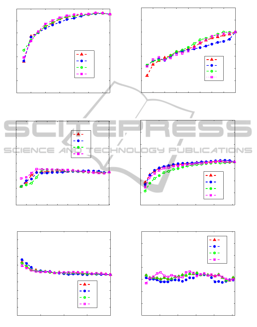
4.3 Accuracy vs. Number of Features

We compare the accuracy rates of the different scores

, C

and C

thanks to our semi-supervised eval-

uation procedure. The labels of the training data are

estimated by the constrained K-means algorithm op-

erating in the selected feature space. These estimated

labels are then used by the nearest neighbor classi-

ﬁer in order to measure the accuracy of the different

scores.

Figure 2 shows the accuracy rates vs the de-

sired number of selected features on the databases

of ’Wine’,’Image segmentation’, ’Vehicle’, ’ORL’,

’Colon cancer’ and ’Leukemia.

From this ﬁgure, we can see that the accuracy rates

of C

, C

and C

are very close, because the dif-

ferent curves overlap. Since these results are averaged

over 100 runs, it is hard to compare them.

That leads us to compare these scores by exam-

ining their accuracies at each of the 100 runs. For a

ﬁxed number of selected features, in each of the 100

runs, we propose to rank the 4 scores in descending

order of their accuracy.

Let us denote rank

∗

the rank of the criterion C

∗

at the run q. This rank takes the values 1, 2, 3 or 4.

At each run q, the score having the highest accuracy

is ranked as 1 and the score with the lowest accuracy

value, is ranked as 4. Scores with the same accuracy

have the same rank.

We calculate the rank sum T

∗

for each semi-

supervised constraint score as follow:

∗

100

∑

q=1

rank

∗

, (9)

where * is 1, 2, 3 or 4 corresponding to the score C

, C

or C

respectively. The method with the low-

est rank sum is considered as being the score which

provides the best results.

Table 1 shows the rank sum T

∗

for the different

databases ’Wine’, ’Image segmentation’, ’Vehicle’,

’ORL’, ’Colon Cancer’ et ’Leukemia’. The rank sum

of each score is computed by considering respectively

the ﬁrst 6, 5, 8, 300, 1000 and 2576 features on the

’Wine’, ’Image segmentation’, ’Vehicle’ and ’ORL’

databases.

Our score C

has the lowest value 3 times (indi-

cated as bold) over the 6 rows of table 1. The other

three scores share each one a row.

SEMI-SUPERVISED EVALUATION OF CONSTRAINT SCORES FOR FEATURE SELECTION

179

0 2 4 6 8 10 12

0.3

0.4

0.5

0.6

0.7

0.8

0.9

Number of selected features

Accuracy

(a) ’Wine’.

0 2 4 6 8 10 12 14 16

0.3

0.4

0.5

0.6

0.7

0.8

0.9

Number of selected features

Accuracy

(b) ’Image segmentation’.

0 2 4 6 8 10 12 14 16 18

0.1

0.2

0.3

0.4

0.5

0.6

0.7

0.8

0.9

Number of selected features

Accuracy

0 200 400 600 800 1000

0.3

0.4

0.5

0.6

0.7

0.8

0.9

Number of selected features

Accuracy

(d) ’ORL’.

0 500 1000 1500 2000

0.1

0.2

0.3

0.4

0.5

0.6

0.7

0.8

0.9

Number of selected features

Accuracy

(e) ’Colon Cancer’.

0 1000 2000 3000 4000 5000

0.3

0.4

0.5

0.6

0.7

0.8

0.9

Number of selected features

Accuracy

(f) ’Leukemia’.

Figure 2: Accuracy rates vs. the desired number of selected features on the 6 databases. 10 constraints composed of 5

must-link et 5 cannot-link was used for the ’Wine’, ’Image segmentation’, ’Vehicle’ and ’ORL’ databases and 60 constraints

composed of 30 must-link and 30 cannot-link was used for the ’Colon Cancer’ and ’Leukemia’ databases. The evaluation is

performed in a semi-supervised learning context: the one nearest neighbor classiﬁer uses the estimated labels of the training

samples as prototypes of classes.

NCTA 2011 - International Conference on Neural Computation Theory and Applications

180

Table 1: The rank sum of the constraint scores on different

databases.

Database \T T

’Wine’ 191 277 206 157

’Image segmentation’ 165 219 161 196

’Vehicle’ 261 239 238 209

’ORL’ 230 200 264 228

’Colon Cancer’ 150 216 162 150

’Leukemia’ 140 240 140 176

These results show that the features selected by

provide accuracy rates that are higher than those

obtained by features selected by the classical scores.

This same conclusion was found in our earlier work

that follows the classical supervised evaluation of the

constraint scores (Kalakech et al., 2011) (Kalakech

et al., 2010).

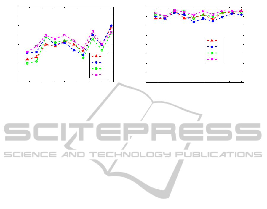
4.4 Accuracy vs. Number of

Constraints

We compare the accuracy rates of the different scores

with a ﬁxed number of features vs. number of pair-

wise constraints.

Figure 3 displays the plot of accuracy with a ﬁxed

number of selected features (half of the number of

original features (Sun and Zhang, 2010) vs. differ-

ent number of pairwise constraints on the two gene

expression databases. The accuracy of the test sam-

ples is measured thanks to the supervised evaluation

scheme.

From this ﬁgure, we can see that, for almost all the

number of constraints, our score C

provides higher

accuracy than C

, C

and C

. We can also notice that

the accuracy does not tend to increase with respect

to the number of constraints. This is due to the con-

straints choice. Since these constraints are randomly

generated, some of them could be less informative

than the others.

Table 2: The rank sum of the constraint scores for different

number 2l of constraints on the ’Colon Cancer’ database.

2l\T T

4 constraints 140 157 153 224

10 constraints 242 147 201 153

40 constraints 153 268 169 124

60 constraints 257 171 194 151

Furthermore, Tables 2 and 3 show the rank sum

∗

for different number 2l of constraints (4, 10, 40

and 60) on the ’Colon Cancer’ and the ’Leukemia’

databases, respectively. The rank sum of each of the

semi-supervised criteria is calculated with the half of

the original features of each of the gene expression

Table 3: The rank sum of the constraint scores for different

number 2l of constraints on the ’Leukemia’ database.

2l\T T

4 constraints 194 215 210 190

10 constraints 234 176 159 150

40 constraints 148 198 196 123

60 constraints 167 170 184 115

databases.

We can see that, for the ’Colon Cancer’ database,

our score provides the lowest rank sum T (indicated

in bold) for 2 times over the 4 rows of Table 2 (when

the number of constraints is higher than 10). For the

’Leukemia database’, our score provides the lowest

rank sum T (indicated in bold) for the different num-

bers of constraints (4, 10, 40 and 60). These results

show that the features selected thanks to our score C

provide accuracy rates which are higher than those

obtained by the features selected by constraint scores

, C

and C

. The same conclusions were found

using the classical supervised evaluation (Kalakech

et al., 2011).

5 CONCLUSIONS

The accuracy rates of test samples reached by a clas-

siﬁer that analyses the features selected by the con-

straint scores, are generally compared in the super-

vised learning context. The nearest neighbor clas-

siﬁer uses the training sample labels as prototypes

of classes. However, the feature selection has been

performed in a semi-supervised context, since it uses

the available constraint sets and/or the unconstrained

samples.

So, we have proposed in this paper, to keep the

same learning context for the feature selection as for

the evaluation. The prior knowledge represented by

must-link and cannot-link constraints is used for the

selection and for the classiﬁcation. The training sam-

ple labels are estimated by using the constrained K-

means algorithm that tries to respect the constraints

as much as possible. These estimated labels are then

used as prototypes by the nearest neighbor classiﬁer

to classify the test samples. We called this approach

semi-supervised evaluation to distinguish it from the

classical supervised one.

The comparison between the different constraint

scores thanks to this semi-supervised evaluation

shows that the accuracy rates provided by our score

are higher than those of the classical scores.

We notice that the constrained K-means used dur-

ing the semi-supervised evaluation is a simple cluster-

ing algorithm. It does not guarantee the respect of all

SEMI-SUPERVISED EVALUATION OF CONSTRAINT SCORES FOR FEATURE SELECTION

181

0 5 10 15 20 25 30 35 40

0.3

0.35

0.4

0.45

0.5

0.55

0.6

0.65

Number of constraints

Accuracy

(a) ’Colon Cancer’.

0 5 10 15 20 25 30 35 40

0.3

0.35

0.4

0.45

0.5

0.55

0.6

0.65

Number of constraints

Accuracy

(b) ’Leukemia’.

Figure 3: Accuracy rates vs. number of constraints for C

, C

and C

on the gene expression databases thanks to the

semi-supervised evaluation scheme. The desired number of selected features is half of the number of the original features.

the constraints specially when several constraints are

deﬁned with the same sample. So, it will be interest-

ing to use another constrained classiﬁcation algorithm

that is more efﬁcient than this one, as these presented

by Kulis et al. (Kulis et al., 2009) and Davidson et al.

(Davidson et al., 2006).

REFERENCES

Alon, U., Barkai, N., Notterman, D., Gishdagger, K., Ybar-

radagger, S., Mackdagger, D., and Levine, A. (1999).

Broad patterns of gene expression revealed by cluster-

ing analysis of tumor and normal colon tissues probed

by oligonucleotide arrays. Proceedings of the Na-

tional Academy of Science of the USA, 96(12):745–

6750.

Blake, C., Keogh, E., and Merz, C. (1998). UCI

repository of machine learning databases.

http://www.ics.uci.edu/ mlearn/MLRepository.html.

Carpaneto, G. and Toth, P. (1980). Algorithm 548: solu-

tion of the assignment problem. ACM Transactions

on Mathematical Software.

Davidson, I., Wagstaff, K., and Basu, S. (2006). Measur-

ing constraint-set utility for partitional clustering al-

gorithms. In In proceedings of the Tenth European

Conference on Principles and Practice of Knowledge

Discovery in Databases ’PKDD06’, pages 115–126,

Berlin, Germany.

Golub, T. R., Slonim, D. K., Tamayo, P., Huard, C., Gaasen-

beek, M., Mesirov, J. P., Coller, H., Loh, M. L., Down-

ing, J. R., Caligiuri, M. A., and Bloomﬁeld, C. D.

(1999). Molecular classiﬁcation of cancer: class dis-

covery and class prediction by gene expression moni-

toring. Science, 286:531–537.

He, X., Cai, D., and Niyogi, P. (2005). Laplacian score

for feature selection. In Proceedings of the Advances

in Neural Information Processing Systems (’NIPS

05’), pages 507–514, Vancouver, British Columbia,

Canada.

Kalakech, M., Biela, P., Macaire, L., and Hamad, D. (2011).

Constraint scores for semi-supervised feature selec-

tion: A comparative study. Pattern Recognition Let-

ters, 32(5):656–665.

Kalakech, M., Porebski, A., Biela, P., Hamad, D., and

Macaire, L. (2010). Constraint score for semi-

supervised selection of color texture features. In Pro-

ceedings of the third IEEE International Conference

on Machine Vision (ICMV 2010), pages 275–279.

Kudo, M. and Sklansky, J. (2000). Comparison of algo-

rithms that select features for pattern classiﬁers. Pat-

tern Recognition, 33(1):25–4.

Kulis, B., Basu, S., Dhillon, I., and Mooney, R. (2009).

Semi-supervised graph clustering: a kernel approach.

Machine Learning, 74(1):1–22.

Liu, H. and Motoda, H. (1998). Feature extraction con-

struction and selection a data mining perspective.

Springer, ﬁrst edition.

Samaria, F. and Hartert, A. (1994). Parameterisation of

a stochastic model for human face identiﬁcation. In

Proceedings of the Second IEEE Workshop on Appli-

cations of Computer Vision ’ACV 94’, pages 138–142,

Sarasota, Florida.

Sun, D. and Zhang, D. (2010). Bagging constraint score

for feature selection with pairwise constraints. Pattern

Recognition, 43:2106–2118.

Wagstaff, K., Cardie, C., Rogers, S., and Schroedl, S.

(2001). Constrained k-means clustering with back-

ground knowledge. In Proceedings of the Eigh-

teenth International Conference on Machine Learning

’ICML 01’, pages 577–584, Williamstown, MA, USA.

Zhang, D., Chen, S., and Zhou, Z. (2008). Constraint score:

A new ﬁlter method for feature selection with pairwise

constraints. Pattern Recognition, (41):1440–1451.

Zhao, J., Lu, K., and He, X. (2008). Locality sensitive semi-

supervised feature selection. Neurocomputing, 71(10-

12):1842–1849.

Zhao, Z. and Liu, H. (2007). Semi-supervised feature selec-

tion via spectral analysis. In Proceedings of the SIAM

International Conference on Data Mining ’ICDM 07’,

pages 641–646, Minneapolis.

NCTA 2011 - International Conference on Neural Computation Theory and Applications

182