
A STATE-SPACE NEURAL NETWORK
FOR MODELING DYNAMICAL NONLINEAR SYSTEMS
Karima Amoura
1
, Patrice Wira
2
and Said Djennoune
1
1
Laboratoire CCSP, Universit´e Mouloud Mammeri, Tizi Ouzou, Algeria
2
Laboratoire MIPS, Universit´e de Haute Alsace, 4 Rue des Fr`eres Lumi`ere, 68093 Mulhouse, France
Keywords:
Artificial neural networks, Recurrent network, State space, State estimation, System identification, System
dynamics.
Abstract:
In this paper, a specific neural-based model for identification of dynamical nonlinear systems is proposed. This
artificial neural network, called State-Space Neural Network (SSNN), is different from other existing neural
networks. Indeed, it uses a state-space representation while being able to adapt and learn its parameters. These
parameters are the neural weights which are intelligible or understandable. After learning, the SSNN therefore
is able to provide a state-space model of the dynamical nonlinear system. Examples are presented which show
the capability of the SSNN for identification of multivariate dynamical nonlinear systems.
1 INTRODUCTION
The state-space representation is a very powerful tool
for modeling systems (Gauthier and Kupka, 2001). It
allows the modeling of linear and nonlinear dynami-
cal systems while keeping a temporal representation
of the events. It contains useful information directly
related to physical systems and offers thus very good
possibilities in terms of analyzing systems and plants.
An Artificial Neural Network (ANN) is an assem-
bly of connected neurons where each neuron com-
putes its output as a nonlinear weighted sum of its
inputs. If the parameters of this type of architec-
tures, i.e., the weights of the neurons, are appropri-
ately tuned, then the whole architecture is able to esti-
mate the relationship between input and output spaces
or to mimic the behavior of a plant without consider-
ing any model (Haykin, 1994), (Principe et al., 2000).
Learning is one of the most interesting properties of
the ANNs in the sense that calculating and adjusting
the weights is achieved without modeling the plant
and without any knowledge about it, but only from
examples. Examples are sampled signals measured
from the plant and representative of its behavior. In
this way, ANN are considered as relevant modeling
and approximating tools.
A Multi-Layer Perceptron (MLP) is a neural ar-
chitecture where neurons are organized in layers. Be-
side, a Recurrent Neural Network (RNN) can be con-
sidered as a MLPs enhanced by feedback connec-
tions. RNNs are considered a cornerstone in the learn-
ing theory because of their abilities to reproduce dy-
namical behaviors by mean of feedback connections
and delays in the propagation of their signals (El-
man, 1990). After learning, a RNN with a sufficient
number of neurons is able to estimate any relation-
ships and therefore to reproduce the behavior of any
multivariate and nonlinear dynamical systems (Wer-
bos, 1974). Therefore, RNNs received a consider-
able attention from the modern control community
to such an extend that they have been formalized
in Model-Referencing Adaptive Control (MRAC)
schemes (Narendra and Parthasarathy, 1990), (Chen
and Khalil, 1992). Their model stability remains one
of the most critical aspects.
The deterministic state-space representation and
the learning RNN can both be employed for modeling
dynamical systems. However, they are characterized
by very different ways of storing information. If the
first approach directly relies on physical parameters
of the system, the second approach uses the weights
of the neurons. These weights are inherent of a neu-
ral architecture and can generally not be interpreted.
Combining these two approaches would combine the
advantages of one and the other. This is the case ofthe
State-Space Neural Network (SSNN), a very specific
RNN based on a state-space representation (Zamar-
reno and Vega, 1998).
In this paper, the SSNN is proposed for the identi-
fication of multivariate nonlinear dynamical systems.
369
Amoura K., Wira P. and Djennoune S..
A STATE-SPACE NEURAL NETWORK FOR MODELING DYNAMICAL NONLINEAR SYSTEMS.
DOI: 10.5220/0003680503690376
In Proceedings of the International Conference on Neural Computation Theory and Applications (NCTA-2011), pages 369-376
ISBN: 978-989-8425-84-3
Copyright
c
2011 SCITEPRESS (Science and Technology Publications, Lda.)

The architecture of the SSNN differs from conven-
tional neural architectures by being compliant to a
state-space representation. Indeed, the SSNN is de-
voted to approximate the nonlinear functions between
the input, state, and output spaces. It is therefore a
state-space formalism enhanced by learning capabil-
ities for adjusting its parameters. Its state represen-
tation is accessible and can be used moreover for the
design of adaptive control schemes. Previous RNN-
based approaches (Kim et al., 1997), (Mirikitani and
Nikolaev, 2010) can be good candidates for yielding
adaptive observers. However, they are restricted to
some classes of nonlinear systems. On the other hand,
the SSNN is able to describe virtually any nonlinear
system dynamics with a state-space representation. It
is therefore of a considerable interest for identification
and control purposes.
The paper is organized as follows. In Section II,
the SSNN equations are developed. Two simulation
examples are provided in Section III to illustrate and
to compare the performance of the SSNN used for the
system identification of nonlinear plants. Some con-
cluding remarks are provided at the end of the paper.
2 THE STATE-SPACE NEURAL
NETWORK (SSNN)
2.1 Architecture
The general formulation of a discrete-time process
governed by a nonlinear difference equation can be
written by
x(k+ 1) = F(x(k), u(k))
y(k) = G(x(k)) + v(k)
. (1)
The evolution of the process is represented by its
internal state x ∈ R
s
. The process takes the control
signals u ∈ R
n
as the inputs and outputs measure-
ments y ∈ R
m
. F and G are nonlinear multivariate
functions representing the process nonlinearities.
The SSNN is a special RNN whose architecture
exactly mirrors a nonlinear state-space representation
of a dynamical system (Zamarreno and Vega, 1998;
Zamarreno and Vega, 1999; Zamarreno et al., 2000;
Gonzalez and Zamarreno, 2002). The SSNN is com-
posed of five successive layers: an input layer, a hid-
den layer S, a state layer, a hidden layer O, and an
output layer. The input layer takes the input signals
and delivers them to every neurons of hidden layer S.
This layer describes the states behavior by introduc-
ing a form of nonlinearity. The state layer is com-
posed of neurons receiving the signals from hidden
{
{
input hidden state hidden output
x(k− 1)
u(k)
u(k)
RNA1
x(k)
x(k)
RNA2
y(k)
y(k)
W
i
s
o
W
0
W
h2
W
r
W
h
a)
b)
Figure 1: Architecture of the SSNN, a) the two-stage neural
block representation, b) the SSNN signal flow graph.
layer S as inputs. Each neuron in this layer represents
one state whose output value is an estimated value of
the state. The estimated states are used by the next
hidden layer O which relates the states to the output
layer via a nonlinear function. The output layer is
composed of neurons taking the hidden layer signals
as inputs. The outputs of the neurons composing the
output layer finally representthe outputs of the SSNN.
The SSNN topology can be also considered as a two-
stage architecture with two ANN blocks, ANN1 and
ANN2, separated by an internalestimated state-space.
This architecture is equivalent to a deterministic non-
linear system in a state-space form whose mathemat-
ical representation is a particular case of (1):
ˆx(k+ 1) = W
h
F
1
W
r
ˆx(k) + W
i
u(k) + B
h
+ B
l
ˆy(k) = W
0
F
2
W
h2
ˆx(k) + B
h2
+ B
l2
(2)
where ˆy ∈ R
m
and ˆx ∈ R
s
represent the estimation
of y and x respectively. The other parameters are:
• W
i
∈ R
h
× R
n
, W
h
∈ R
s
× R
h
, W
r
∈ R
h
× R
s
,
W
h2
∈ R
h2
× R
s
and W
0
∈ R
m
× R
h2
are weight-
ing matrices;
• B
h
∈ R
h
, B
h2
∈ R
h2
, B
l
∈ R
s
and B
l2
∈ R
m
are bias
vectors;
• F
1
, R
h
→ R
h
and F
2
, R
h2
→ R
h2
are two static
and nonlinear functions.
The architecture of the SSNN is represented by
the schematic diagram of Fig. 1 a). Its five layers
are represented by the signal flow graph of Fig. 1 b)
where black (or full) nodes are variables linearly de-
pending from the previous ones and where white
(or empty) nodes are variables nonlinearly depend-
ing from the previous ones. Compared to its initial
formulation (Zamarreno and Vega, 1998; Zamarreno
and Vega, 1999; Zamarreno et al., 2000), the form
of (2) has been enhanced with biases B
l
and B
l2
in
NCTA 2011 - International Conference on Neural Computation Theory and Applications
370
order to allow more flexibility to the neural architec-
ture. These additional degrees of freedom will allow
better performances for learning and estimating a pro-
cess. The learning consists in finding the optimal val-
ues of the weights and biases. The parameters fixed
by the designer are the functions F
1
and F
2
, and the
initial values
ˆ
x(0). It is important to notice that: 1)
the SSNN needs an initial state value, 2) the numbers
of inputs and outputs of the SSNN (therefore n and
m respectively) are fixed by those of the plant to be
modeled, 3) h and h2, the number of neurons in the
hidden layers, are let to the designer’s appreciation.
The SSNN is able to reproduce the same behavior
as the process with weights and biases correctly ad-
justed. This means that the SSNN is able to yield a
signal
ˆ
y(k) very close to the output y(k) of the pro-
cess for the same control signal u ∈ R
n
. Furthermore,
and contrary to other ANNs, the SSNN is also able
to provide an estimation
ˆ
x(k) of the state x(k) at any
instant k due to its specific architecture. Obviously,
the performance depends on the learning, i.e., if the
parameters have been well adjusted.
2.2 Parameters Estimation
Learning or training addresses the parameters estima-
tion of the neural technique. The problem of interest
consists in using data sets from the system in order
to find the best possible weights so that the ANN re-
produces the system behavior. The learning of the
SSNN is based on the general learning theory for
a feed-forward network with n
′
input and m
′
output
units (Haykin, 1994). It can consist of any number of
hidden units and can exhibit any desired feed-forward
connection pattern.
It is therefore a nonlinear optimization problem
based on a cost function which must be defined to
evaluate the fitness or the error of a particular weight
vector. The Mean Squared Error (MSE) of the net-
work is generally used as the performance index and
must be minimized:
E =
1
2
∑
N
k=1
ke(k)k
2
=
1
2
∑
N
k=1
b
y(k) − d
′
(k)
2
,
(3)
with a given training set
{(x
′
(1), d
′
(1)), ..., (x
′
(N), d
′
(N))} consisting of
N ordered pairs of of n
′
- and m
′
-dimensional vectors
which are called the input and output patterns.
The weights of the ANN are adjusted via gradi-
ent descend methods to minimize the MSE between
the desired response d
′
(k) and the actual output
b
y(k)
of the network. Several learning algorithms have
been proposed in the literature (Werbos, 1974), (El-
man, 1990), (Chen and Khalil, 1992), (Principe et al.,
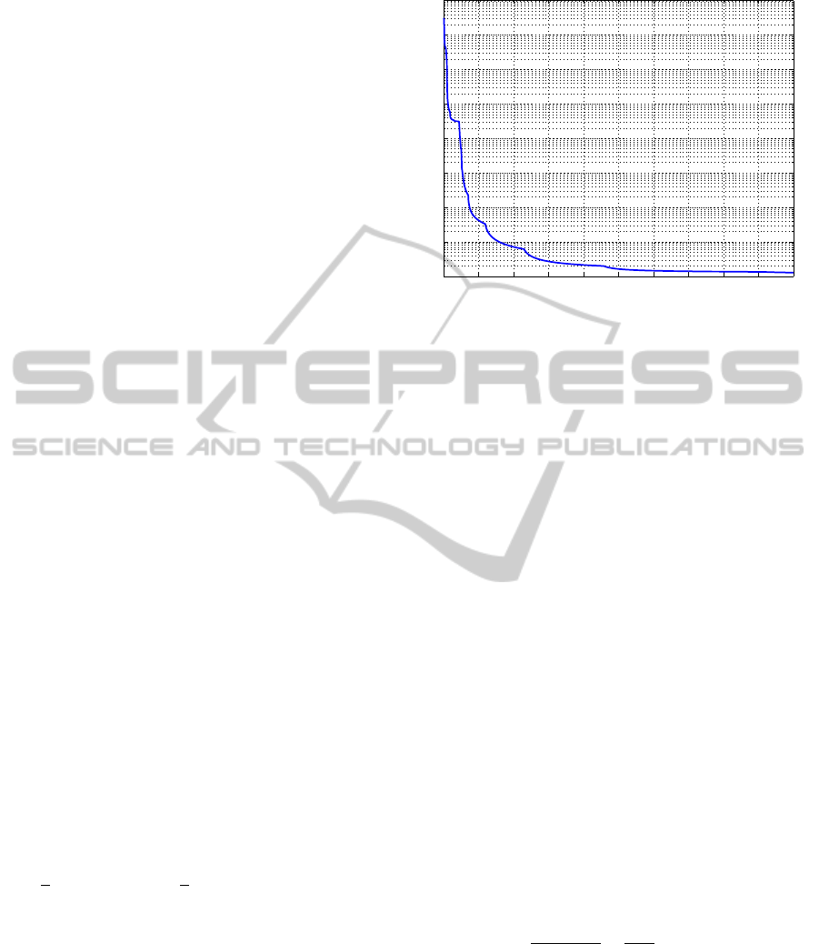
0 100 200 300 400 500 600 700 800 900 1000
10
-7
10
-6
10
-5
10
-4
10
-3
10
-2
10
-1
10
0
10
1
epochs
Performance
Figure 2: MSE values obtained during the training phase
for plant example 1.
2000). The backpropagation algorithm with the
Levenberg-Marquardt method is used to find a min-
imum for the MSE. The network is initialized with
weights randomly chosen between -1 and 1.
In the SSNN, we assume that ANN1 and ANN2
of are trained with this principle by using respec-
tively
n
...,
u(k)
b
x(k− 1)
T
, s(k)
, ...
o
and
{..., (s(k), y(k)), ...} for their training sets.
3 SIMULATION TESTS
AND RESULTS
In this study, the SSNN is applied to system identi-
fication of two multivariate nonlinear dynamical sys-
tems in order to evaluate and to compare its perfor-
mance. Indeed, it is used to learn a state-space repre-
sentation of these systems.
3.1 Example 1
We consider the following process, governed by a de-
terministic second-order nonlinear state-space repre-
sentation:
x
1
(k+ 1) = 1.145x
1
(k) + 0.549x
2
(k) + 0.584u(k)
x
2
(k+ 1) =
x
1
(k)
1+0.01x
2
2
(k)
+
0.181
0.549
u(k)
y(k) = 4tanh(0.250x
1
(k))
(4)
with the state vector x(k) =
x
1
(k) x
2
(k)
T
and a
one dimensional control signal u(k).
This process is estimated by a SSNN with acti-
vation functions F
1
and F
2
that are respectively sig-
moid type and tanh-type. The other parameters are
n=1, s = 2, and m = 1. The number of neurons in
A STATE-SPACE NEURAL NETWORK FOR MODELING DYNAMICAL NONLINEAR SYSTEMS
371
the hidden layers of ANN1 and ANN2 are fixed by a
trial-and-errorprocess and the best performanceis ob-
tained with h = h2 = 2 neurons in each hidden layer.
The initial conditions of the SSNN are the following:
the weights are randomly chosen between -1 and 1,
and
ˆ
x(0) is chosen as null. In order to train the SSNN,
1800 training inputs are generated with a sinusoidal
control signal with different values of the amplitude
and frequency. The training error values vs. the num-
ber of epochs are shown in Fig. 2.
After learning with the Levenberg-Marquardt al-
gorithm, the plant described by (4) is estimated by
the SSNN according to
ˆx(k + 1) = W
h
logsig
W
r
ˆx(k) + W
i
u(k) +B
h
+ B
l
ˆy(k) = W
0
tansig
W
h2
ˆx(k) + B
h2
+ b
l2
(5)
with the following optimum weights:
W
r
=
−0.0340 0.0162
−0.2375 −0.2529
,
W
h
=
−134.8114 0.0261
−81.8352 −5.2239
,
W
i
=
−0.0173 0.0211
T
,
B
h
=
−0.0023 −0.0001
T
,
B
l
=
67.3160 43.4829
T
,
W
h2
=
−5.6543 2.3457
,
W
0
=
−0.500 0.0000
0.500 0.0000
,
B
h2
=
0.1812 0.4369
T
.10
−3
,
b
l2
= 1.6543.
(6)
The SSNN with the previous parameters is evalu-
ated on a test sequence. This allows to compare the
behavior of the SSNN to those of the plant by using
a same control signal composed of steps with various
amplitudes. The results are presented by Fig. 3 which
shows the control input, the two states, the output and
the estimated states and output. This figure shows at
the same time, the different between the output and its
estimation and the difference between the states and
their estimation. The maximum value of the MSE on
the output of the SSNN is 25 .10
−6
; this demonstrates
the ability of the SSNN for modeling this nonlinear
dynamical plant.
3.2 Example 2
In this example, the plant to be identified is a four-
order nonlinear system (s = 4) with m = 4 outputs:
0 50 100 150 200 250 300
-4
-2
0
2
4
(p.u.)
x
2
ˆx
2
0 50 100 150 200 250 300
-4
-2
0
2
4
(p.u.)
x
1
ˆx
1
0 50 100 150 200 250 300
-3
-2
-1
0
1
2
3
(p.u.)
y
ˆ
y
0 50 100 150 200 250 300
-0.03
-0.02
-0.01
0
0.01
0.02
0.03
time (iterations)
errors (p.u.)
y − ˆy
u
ˆx
1
x -
1
ˆx
2
x -
2
Figure 3: Performances of the SSNN in identifying plant
example 1.
x
1
(k+ 1)
x
2
(k+ 1)
x
3
(k+ 1)
x
4
(k+ 1)
=
x
2
(k)
psinx
1
(k) + p+ x
3
(k)
x
4
(k)
px
3
(k)
+
0
0
0
1
u(k)
y(k) = tanh(x(k))
(7)
where parameter p = 0.85. The plant is linear with
p = 0, nonlinear with p > 0, and unstable with p ≥ 1.
The plant is controlled by one input signal u (there-
fore n = 1) which is a sinusoidal signal with differ-
ent values of the period, mean (offset) and ampli-
tude. The training set of the SSNN is composed of
1000 data samples of u, y, and x). The plant non-
linearities are introduced in the SSNN with functions
F
1
(.) = logsig(.) and F
2
(.) = tansig(.). For simplic-
ity, the following initial conditions are considered:
x(0) = 0 and
ˆ
x(0) = 0. The parameters of the SSNN
are randomly initialized between -1 and 1 and are
adjusted with the training data set according to the
Levenberg-Marquardt algorithm.
After learning ex-nihilo, the plant of (7) is identi-
fied by
ˆx(k+1) = W
h
logsig
W
r
ˆx(k) + W
i
u(k) + B
h
+ B
l
ˆy(k) = W
0
tansig
W
h2
ˆx(k) + B
h2
+ B
l2
(8)
NCTA 2011 - International Conference on Neural Computation Theory and Applications
372
0 200 400 600 800 1000 1200 1400 1600 1800
−4
−2
0
2
0 200 400 600 800 1000 1200 1400 1600 1800
−20
−10
0
10
20
0 200 400 600 800 1000 1200 1400 1600 1800
−2
−1
0
1
2
u
y
ˆy
x
ˆx
Figure 4: Test sequence of the SSNN with an oscillating
control signal.
The best results for the SSNN are obtained with
h = 8 and h2 = 4 with the following values:
W
r
=
0.0001 0.0211 0.0209 −0.0312
0.7841 −0.0345 −0.0740 0.1457
0.5381 0.0135 −0.0937 0.0806
−0.2618 0.0035 0.0632 −0.0544
−0.0001 −0.0198 0.0150 −0.0128
−0.4081 −0.0045 0.0763 −0.0678
−0.0000 −0.0195 0.0075 0.0199
0.6801 0.0027 −0.0052 0.0534
,
W
h
=
91.3394 27.7993 34.2220 127.4106
0.0043 20.4352 −0.0179 −0.0017
0.0563 −230.9712 0.2334 0.1122
0.1380 321.3377 −0.2097 −0.0990
−151.3135 −49.3097 −131.2520 −37.2734
0.0636 −501.6847 0.4946 0.2431
46.5102 106.5639 169.5512 175.2242
−0.0046 23.6573 −0.0277 −0.0094
T
W
i
=
0.0247
−0.1018
−0.0217
0.0102
0.0176
0.0179
0.0087
−0.0639
, B
h
=
−0.0409
−10.0577
−1.6909
0.7563
0.0391
1.2601
0.0029
4.5821
,
B
l
=
h
8.9622 143.6209 −35.0017 −131.2700
i
T
,
W
h2
=
31.3282 −16.9499 −39.0042 25.6931
−0.0323 0.0403 −1.0431 0.0221
−0.0284 0.0387 0.0360 0.9379
−0.5062 −0.4215 0.0543 −0.0515
,
W
0
=
0.0651 −0.0354 −0.1039 −1.0478
−0.0697 0.0862 0.1236 −0.9888
−0.0029 −0.9360 0.0519 −0.0130
0.0016 0.0042 1.0206 0.0171
T
,
B
h2
=
9.3989
0.0074
0.0083
0.0159
, B
l2
=
−0.0583
0.0601
0.0036
−0.0031
T
.
(9)
First, we report results for a test sequence based
0 200 400 600 800 1000 1200 1400 1600 1800
−0.4
−0.3
−0.2
−0.1
0
0.1
0.2
0.3
x − ˆx
0 200 400 600 800 1000 1200 1400 1600 1800
−0.5
0
0.5
y − ˆy
Figure 5: Estimating errors of the SSNN during the test se-
quence.
on an oscillating control signal u ∈ [−3, 2] composed
of 1800 data points. Fig. 4 shows the control signal
u, but also x, y,
ˆ
x, and
ˆ
y. The estimation errors x−
ˆ
x
and y−
ˆ
y are presented by Fig. 5. The performance in
estimating the plant with the SSNN can also be eval-
uated by the MSE and the maximum error on x and
ˆ
y
reported in the left part of Table 1 (test sequence). It
can be seen from this table that the maximum error is
less than 1.4% in estimating the states and less than
22.5% in estimating the output. The greatest errors
are recorded on the transcients and the static error is
negligible compared to the range of the output.
In order to go further into the SSNN estimation ca-
pabilities, we evaluate its response to a step and com-
pare it to the original plant. Fig. 6 shows the states
of the SSNN and of the plant. Fig. 7 shows the out-
puts of the SSNN and of the plant. It can be seen that
the behavior of the SSNN is very close to the one of
the plant. This is confirmed by the errors, i.e., MSE
and static errors reported in the right part of Table 1
(step response). In this test, the behavior of the SSNN
is nearly the same as that of the plant, all the more
so since the training sequence of the SSNN was not
composed of steps but only of sinusoidal waves. This
demonstrates that the SSNN is successful in identifi-
cation and its the good capabilities to generalize.
If system identification includes estimating the re-
lation between the input and the output of the system,
this can be achieved by a MLP and can be used as a
comparison to the SSNN. Fig. 8 shows the principle
of identifying a plant with a MLP using delayed in-
put and output signals. The input of the MLP are de-
layed values of the control signal u(k) and of the out-
put of the process y(k) in order to capture the process
dynamics. We chose to update the MLP weights ac-
cording to the Levenberg-Marquardt algorithm from
a random initialization between -1 and 1 and with the
A STATE-SPACE NEURAL NETWORK FOR MODELING DYNAMICAL NONLINEAR SYSTEMS
373
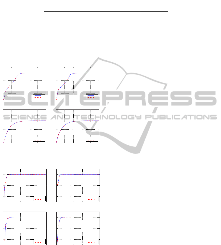
Table 1: SSNN errors in identifying plant example 2.
test sequence step response
MSE max. error MSE static error
x
1
0.0007 10
−3
0.0157 0.2177 10
−3
-0.1246
x
2
0.5228 10
−3
0.3474 0.3753 10
−3
-0.1155
x
3
0.0014 10
−3
0.0141 0.0297 10
−3
-0.2084
x
4
0.0012 10
−3
0.0088 0.0237 10
−3
-0.1995
y
1
0.0031 10
−3
0.4145 0.4535 10
−3
-0.1105
y
2
0.0034 10
−3
0.4495 0.5477 10
−3
-0.1027
y
3
0.0000 10
−3
0.0259 0.0078 10
−3
-0.1998
y
4
0.0000 10
−3
0.0386 0.0113 10
−3
-0.1998
0 20 40 60 80 100
0
2
4
6
8
10
0 20 40 60 80 100
0
2
4
6
8
10
0 20 40 60 80 100
0
2
4
6
8
10
0 20 40 60 80 100
0
2
4
6
8
10
x
1
ˆx
1
x
2
ˆx
2
x
3
ˆx
3
x
4
ˆx
4
temps (itérations) temps (itérations)
(sans unité)
(sans unité)
(sans unité)
(sans unité)
temps (itérations) temps (itérations)
Figure 6: Ideal states and states estimated by the SSNN for
an input step (plant example 2).
0 10 20 30 40 50
0
0.2
0.4
0.6
0.8
1
1.2
0 10 20 30 40 50
0
0.2
0.4
0.6
0.8
1
1.2
0 10 20 30 40 50
0
0.2
0.4
0.6
0.8
1
0 10 20 30 40 50
0
0.2
0.4
0.6
0.8
1
y
1
ˆy
1
y
2
ˆy
2
y
3
ˆy
3
y
4
ˆy
4
temps (itérations) temps (itérations)
(sans unité)
(sans unité)
(sans unité)
(sans unité)
temps (itérations) temps (itérations)
Figure 7: Ideal outputs and outputs estimated by the SSNN
for an input step (plant example 2).
same training set as for the SSNN. After the training
period, the MLP has been evaluated with the same test
sequence as for the SSNN and with a step response.
Results obtained with a MLP that uses 10 scalar in-
puts (i.e., u(k), u(k−1), y(k) and y(k−1)), 8 neurons
in one hidden layer and 4 outputs are presented in Ta-
ble 2. They can be compared to the ones obtained
with the SSNN in Table 1. The errors of the MLP and
of the SSNN in yielding the output are of the same
order of magnitude. However, the MLP is a nonlinear
regression structure that represents input-output map-
pings by weighted sums of nonlinear functions. The
MLP is therefore not able to estimate the state signals
of the plant.
3.3 Discussion
Computational cost is generally considered as a ma-
jor shortcoming of ANNs when identifying and con-
trolling dynamical systems in real-time. Their main
interest is to used an on-line learning, i.e., to adjust
the weights while controlling of the system at the
same time. This means that both, learning and con-
trolling, are achieved within each iteration. This al-
lows to instantaneously take into account the varia-
tions and fluctuations of the system’s parameters and
the eventual external disturbances affecting the sys-
tem. The computational costs for calculating the out-
put and updating the weights have to be compatible
with the sampling time.
The number of neurons is generally provided to
give an idea about the size of the ANN. The num-
ber of neurons is h + s + h2 + m for a SSNN noted
down by SSNN(n, h, s, h2, m) with n, h, s, h2 and
m, the dimensions of the SSNN five successive lay-
ers. The number of neurons is m2 + m3 for a MLP
with m1 inputs, m2 neurons in one hidden layer, and
m3 outputs, i.e., MLP(m1, m2, m3). In example 2,
the followingdimensions were imposed on the SSNN,
n = 1, s = m = 4 and m1 = 10 and m3 = 4 on the
MLP. Very close performances were obtained with
SSNN(1,8,4,4,4) and MLP(10,8,4), i.e., respectively
with 20 and 12 neurons. However, this number is not
really representative of the memory required for the
implementation. The total number of scalar param-
eters is much more significant and can be calculated
for the MLP and for the SSNN respectively as general
NCTA 2011 - International Conference on Neural Computation Theory and Applications
374

Table 2: MLP errors in identifying plant example 2.
test sequence step response
MSE max. error MSE static error
y
1
0.0045 10
−3
0.0199 0.3995 10
−3
-0.1087
y
2
0.0047 10
−3
0.0175 0.5021 10
−3
-0.1012
y
3
0.0038 10
−3
0.0166 0.0066 10
−3
-0.1988
y
4
0.0039 10
−3
0.0169 0.0830 10
−3
-0.1907
ANN
plant
+
-
u(k)
y(k)
z
−1
, ..., z
−d
z
−1
, ..., z
−d
e(k)
Figure 8: Typical identification of a plant with a ANN.
functions of the number of hidden neurons by
p
MLP
= f(m2) = (1+ m1+ m3)m2 + m3,
p
SSNN
= f(h, h2)
= (1+ n+ 2s)h + (1+s+ m)h2+ s+ m.
More specifically, for plant example 2, p
SSNN
=
10 h + 9 h2 + 8 and p
MLP
= 15 m2 + 4. With h = 8
and h2 = 4 for the SSNN and with m2 = 8 for the the
MLP, both approaches present the same error in iden-
tification and with the same number of parameters to
be adjusted (124) but respectively with 20 and 12 neu-
rons. This means that a SSNN which uses 20 neurons
is equivalent in terms of performance and of memory
size than a MLP with 12 neurons.
Finally, we evaluate the computational coast of
both neural approaches by specifying the number of
scalar operations involved for calculating the esti-
mated output. Calculating the output of a simple
neuron with m1 inputs and 1 bias requires m1 scalar
multiplications, m1 scalar additions and the process-
ing through 1 scalar nonlinear function. This general
fact can be noted down by m1⊗ +m1 ⊕ +1f. Cal-
culating the output of MLP(m1, m2, m3), means to
“propagate” the inputs signals through each neurons
of all the successive layers. The number of the con-
sidered scalar operations is therefore: m2(m1+m3)⊗
+m2(m1 + m3) ⊕ +(m2 + m3) f. We determine the
number of scalar operations for calculating the out-
put of the SSNN as (nh + 2sh+ sh2+ oh2) ⊗ +(nh+
2sh+ sh2+ oh2) ⊕ +(h+ s+ h2+ o) f.
For the specific case of plant example 2,
MLP(10,8,4) needs 112 ⊗ +112 ⊕ +12f while
SSNN(1,8,4,4,4) requires only 104 ⊗ +104⊕ +20f.
The number of scalar operations for the training are
not detailed here because it depends on the gradi-
ent method that is used. Adapting the weights for
the SSNN generally requires less efforts than for the
MLP.
Learning with MLPs remains to estimate the
input-output relationship of a system. This is a way
to describe the system dynamics when conventional
tools are not efficient in modeling. However, MLPs
generally needs a substantial number of time-delayed
signals as additional inputs to efficiently capture the
system dynamics. This means a large number of
weights and therefore introduces some difficulties in
its learning convergence(Haykin, 1994). On the other
side, the SSNN outdoes the simple input-output re-
lationship estimation problem. Its captures the sys-
tem dynamics with an architecture that inherently
mirrors a state-space representation. The SSNN al-
lows the reconstruction of a state space and gives
access to the states values. The numerical values
presented here shows that, compared to a MLP, the
SSNN presents the best compromise between com-
putational resources and performances. The SSNN is
more compliant to real-time constraints than the MLP.
Accordingly, the SSNN is well suited to adaptivecon-
trol schemes based on state-space representations.
4 CONCLUSIONS
In this paper, a State-Space Neural Network (SSNN)
is evaluated for modeling dynamical nonlinear sys-
tems. This neural approach is a particular type of a
recurrent neural network based on a state-space rep-
resentation. After learning from example data, the
SSNN allows the reconstruction of a state-space rep-
resentation of any nonlinear system. Furthermore, the
SSNN is also able to followthe evolution of the states.
The effectiveness of the SSNN has been illustrated by
simulation examples and results demonstrate the ef-
fectiveness of this adaptive observer. These examples
verify the accuracy of the SSNN in modeling multi-
variate dynamical and nonlinear plants. Finally, the
SSNN is compared to a rough implementation of a
Multi-Layer Perceptron and a thorough study of all
the scalar operations and memory sizes of the two ap-
proaches shows that the SSNN uses reduced compu-
A STATE-SPACE NEURAL NETWORK FOR MODELING DYNAMICAL NONLINEAR SYSTEMS
375

tational costs while allowing the same estimation per-
formance or better parameter tracking capability for
the same computational costs.
REFERENCES
Chen, F. and Khalil, H. (1992). Adaptive control of non-
linear systems using neural networks. International
Journal of Control, 55(6):1299–1317.
Elman, J. (1990). Finding structure in time. Cognitive Sci-
ence, 14(2):179–211.
Gauthier, J.-P. and Kupka, I. (2001). Deterministic obser-
vation theory and applications. Cambridge University
Press, Cambridge, UK.
Gonzalez, P. A. and Zamarreno, J. M. (2002). A short-term
temperature forecaster based on a state space neural
network. Engineering Applications of Artificial Intel-
ligence, 15(5):459–464.
Haykin, S. (1994). Neural Networks : A comprehensive
Foundation. Macmillan College Publishing Company,
Inc., New York.
Kim, Y. H., Lewis, F. L., and Abdallah, C. T. (1997). A
dynamic recurrent neural-network-based adaptive ob-
server for a class of nonlinear systems. Automatica,
33(8):1539–1543.
Mirikitani, D. and Nikolaev, N. (2010). Recursive bayesian
recurrent neural networks for time-series modeling.
IEEE Transactions on Neural Networks, 21(1):262 –
274.
Narendra, K. and Parthasarathy, K. (1990). Identifica-
tion and control of dynamical systems using neural
networks. IEEE Transactions on Neural Networks,
1(1):4–27.
Principe, J. C., Euliano, N. R., and Lefebvre, W. C. (2000).
Neural and Adaptive Systems: Fundamentals Through
Simulations. John Wiley and Sons.
Werbos, P. (1974). Beyond Regression: New tools for pre-
diction and analysis in the behavioral sciences. Ph.d.
thesis, Harvard University.
Zamarreno, J. and Vega, P. (1998). State space neural net-
work. properties and application. Neural Networks,
11(6):1099–1112.
Zamarreno, J., Vega, P., Garca, L., and Francisco, M.
(2000). State-space neural network for modelling,
prediction and control. Control Engineering Practice,
8(9):1063–1075.
Zamarreno, J. M. and Vega, P. (1999). Neural predic-
tive control. application to a highly non-linear sys-
tem. Engineering Applications of Artificial Intelli-
gence, 12(2):149–158.
NCTA 2011 - International Conference on Neural Computation Theory and Applications
376
