
NEURAL PROCESSING OF LONG LASTING SEQUENCES
OF TEMPORAL CODES
Model of Artificial Neural Network based on a Spike
Timing-dependant Learning Rule
Dalius Krunglevicius
Faculty of Mathematics and Informatics, Vilnius University, Naugarduko 24, LT-03225 Vilnius, Lithuania
Keywords: Artificial neural networks, Spike timing-dependent plasticity, STDP, Hebbian learning, Temporal coding,
Neuroscience.
Abstract: It has been demonstrated, that spike-timing-dependent plasticity (STDP) learning rule can be applied to train
neuron to become selective to a spatiotemporal spike pattern. In this paper, we propose a model of neural
network that is capable of memorizing prolonged sequences of different spike patterns and learn aggregated
data in a larger temporal window.
1 INTRODUCTION
There are strong experimental evidences that at least
some living neural systems exchange information in
almost binary fashion, in so called temporal spike
codes (Prut et al., 1998; Gerstner and Kistler, 2002;
Fellous et al., 2004; VanRullen et al., 2005, Kayser
et al., 2009). Underlying concept of temporal coding
states that precise spike timing encodes the
information processed by neurons. It is an
alternative to an established concept of rate coding,
when count of spikes in certain time window
encodes the information. There are known
prominent models of neural networks based on rate
coding, such as networks based on Bienenstock-
Cooper-Munro (BCM) theory (Bienenstock et al.,
1982). However, there are evidences that rate coding
alone cannot account for the efficiency of
information transmission in some biological neural
systems (Gerstner et al., 1996; VanRullen and
Thorpe, 2001).
Discovery of spike timing-dependant plasticity
(STDP) learning rules strongly advocates in favor of
temporal coding. Some researches refer to STDP as
Hebbian learning, although STDP do not exactly fit
Hebbian postulate. STDP learning rules are well
established biological processes that guard amount
of synaptic strength change depending on time
difference between incoming (presynaptic) and
outgoing (postsynaptic) spikes. There has been
discovered a number of different STDP rules. STDP
rules vary depending on synapse type or even on a
position on a dendrite (Bi and Poo, 1998; Woodin et
al., 2003; Abbott and Nelson, 2000; Caporale and
Dan, 2008).
STDP learning rule that is common to the
excitatory-to-excitatory synapses, in a certain range
of parameters perfectly fits for training of neurons to
respond to a repeated temporal code. There is an
experimental evidence that pyramidal neurons of rat
operates in this range (Feldman, 2000). In this case,
the neuron trained with this STDP rule acts as a
coincidence detector (Abbott & Nelson, 2000).
Unsupervised learning of temporal codes by
applying STDP training has been already explored
by the number of authors (Masquelier et al., 2008,
2009; Song et al., 2000; Guyonneau et al., 2005;
Gerstner and Kistler, 2002).
We focus our research on temporal coding and
STDP learning rule.
In a recent paper Masquelier et al. (Masquelier et
al., 2009) demonstrated winner-takes-all (WTA)
artificial neural network that is capable of learning
multiple spatiotemporal patterns in a noisy
environment. However, such model is capable of
learning only very short patterns in order of a few
milliseconds. Although Masquelier experimented
with 50ms length training sample patterns, neurons
eventually learned only the very beginning of the
pattern or a later part of it if the beginning was
196
Krunglevicius D..
NEURAL PROCESSING OF LONG LASTING SEQUENCES OF TEMPORAL CODES - Model of Artificial Neural Network based on a Spike
Timing-dependant Learning Rule.
DOI: 10.5220/0003681401960204
In Proceedings of the International Conference on Neural Computation Theory and Applications (NCTA-2011), pages 196-204
ISBN: 978-989-8425-84-3
Copyright
c
2011 SCITEPRESS (Science and Technology Publications, Lda.)

occupied by competing neuron. We executed a
similar experiment and found that neurons became
selective only for 1 or 2 milliseconds of the pattern.
The rest of the pattern could be removed or replaced
with a different pattern without any changes in a
neuron selectivity.
It is evident that central neural systems of
humans and many other advanced species are
capable of learning long lasting patterns of sensory
inputs, such as speech signals, observed motion
patterns etc. If STDP training leads neurons to
learning of coincidences of spikes in a window of a
few milliseconds, then how is it possible for neurons
to learn long lasting pattern of dynamic of sensory
input? In other words, how would we train neurons
to learn patterns of occurrences of different temporal
codes?
In this paper we propose the model of
unsupervised artificial neural network with STDP
training rule that is capable of learning prolonged
sequences of different short spatiotemporal patterns.
The model represents itself a combination of two
WTA layers that are similar to the one demonstrated
by Masquelier et al. (Masquelier et al., 2009) and
inner layers for temporal memory and temporal
modulation.
In the early stages of research we did not seek to
achieve high biological realism, rather created a
model that serves as a proof a concept that known
STDP rules alone can lead to learning of long lasting
combinations of spatiotemporal patterns.
2 UNDERLYING BIOLOGICAL
MECHANISMS
2.1 Leaky Integrate-and-fire Neuron
In this section we provide mathematical model of
leaky integrate-and-fire neuron that we used in the
model.
Figure 1: Neuron action potential as a function of time.
Phases of action potential: 1 - resting potential, 2 - initial
depolarization, 3- regenerative depolarization, 4 -
repolarization, 5 - hyperpolarization. During phases 3 and
4 neuron is in period of complete refraction.
Underlying mechanism of neuron action
potential (AP), in other words spike, was explained
by Hodgkin and Huxley (Hodgkin and Huxley,
1952). For readers' convenience we added an
illustration of different phases of action potential,
since we refer to hyperpolarization phase later in this
paper (Fig 1.)
Function of action potential:
()=
∆
−
∆
−
∆
(1)
where Δt = t - t
spike
; constants K
dpl
= 3, K
hpl
= 5 and
W
ap
=40 define the amplitude of the function of
action potential; T
m
=10ms is the membrane time
constant that defines the slope of the
hyperpolarization phase, T
ap
=0.5ms is the constant
that defines the slope of the spike.
We executed our experiments in precision of one
millisecond relative to the function of action
potential, therefore we refer to single iteration of a
simulation as one millisecond.
Synaptic strength w
j
defines amplitude of
postsynaptic potential (PSP) that would be raised in
postsynaptic neuron membrane by presynaptic spike.
Depending on synapse type, postsynaptic potential
can be positive excitatory (EPSP), or negative
inhibitory (IPSP). If the sum of PSP reached
threshold, that would trigger neuron to produce
action potential, in other words to fire a spike (see
Fig. 1).
Function of postsynaptic potential raised by
spike from individual synapse:
(
)
=
∆
1 +
() −
∆
1 +
() (2)
where Δt = t - t
pre
;
φ
= 1 for excitatory synapses and
φ
= -1 for inhibitory; time constant of the synapse
T
s
=2.5ms; membrane time constant T
m
=10ms is the
same as in equation 1. In simulation of the model,
we optimized PSP calculations and instead of
keeping PSP history for each synapse, we used
accumulated exponential slopes in variables κ
m
and
κ
s
. This is simple, but, to our knowledge, novel
approach that helped to economize computing costs.
κ
m
and κ
s
are updated at the moment of each
presynaptic spike. See equations 3 and 4:
NEURAL PROCESSING OF LONG LASTING SEQUENCES OF TEMPORAL CODES - Model of Artificial Neural
Network based on a Spike Timing-dependant Learning Rule
197
(
)
=
(
)
(
)
∆
1 +
(
−1
)
=
(
−1
)
ℎ
(3)
()=
()
()
∆
1 +
( − 1) =
(−1) ℎ
(4)
Here Δt is a time difference between times of
current and previous presynaptic spikes, w
j
prohibited to decay to 0. w
j(t-1)
and w
j(t)
denominates
synaptic strength before and after STDP
modification. Equations 3, 4 can be derived by
solving trivial equation 5, assuming that at zero
point
κ
0
= 0 and t
1
-t
0
= const and t
1
-t
0
= t-t
0
when t
1
= t:
(
)
(
1+
)
+
(
)
=
(
)
(
1+
)
(5)
Neuron membrane potential at any time:
() =
() =
() + () ℎ
(6)
2.2 Spike Timing-dependant Plasticity
STDP rule is a function of time difference between
presynaptic and postsynaptic spikes that guards the
amount of change of synaptic strength. In our model
we used single STDP rule, see Fig. 2. Long-lasting
decrease of synaptic strength is called long term
depression (LTD), lasting increase is called long
term potentiation (LTP).
Figure 2: STDP rule of excitatory synapses (a) STDP as a
function of spike timing difference. Based on Bi and Poo
(Bi and Poo, 1998). (b) Schematic explanation of STDP,
as a function of time difference between times of
presynaptic and postsynaptic neuron spikes.
STDP function used in our model is expressed in
equation 7. Synaptic strength change for excitatory
synapses, where Δt = t
post
- t
pre
:
∆
=
⋅
∆
∆<0
−
⋅
∆
∆> 0
0
∆=0
(7)
Synaptic strength values are limited between
W
min
and W
max
, which in our model, vary depending
on synapse type. To simplify the calculations of
postsynaptic potentials, we prohibited synapses to
decay less than 1*10
-6
. See equations 3 and 4. See
section 0 for A
LTP
, A
LTD
, T
LTP
and T
LTD
constants.
In our model we used closest neighbor rule, that
is only two closest spikes participate in modification
of synaptic strength. Alternatively all-to-all rule
could be used.
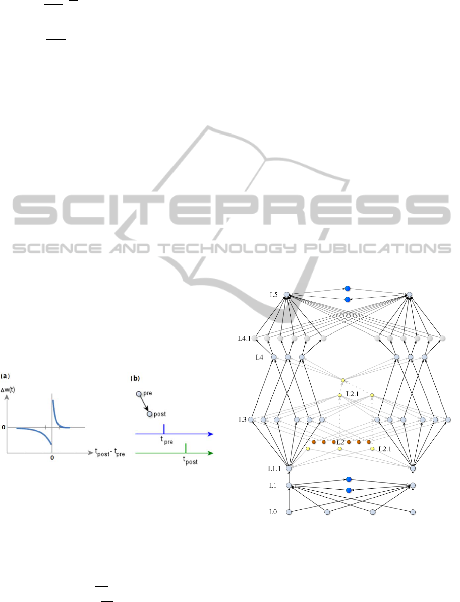
3 THE MODEL
Model diagram is displayed in Fig. 3. It consists of
six main layers: L1 and L5 are competitive
winner(s)-takes-all (WTA) layers (in our model we
did not prohibited a few neurons to learn the same
pattern, therefore we should say winners). L1 and L5
have corresponding inputs from L0 and L4. L3 is a
layer of temporal memory; it is modulated by layer
L2. In our model we did not attempt to match any
layers in cortex or hippocampus, network structure
and layer names are purely arbitrary.
Figure 3: Diagram of the network model with temporal
memory. Blue color denotes inhibitory interneurons. In
real simulation inhibitory neurons are replaced by direct
inhibitory synapses. Grayed lines denote synapses from
L2, L2.1 subnetwork of a temporal modulation. Doted
lines denote that it is the same neuron, split in a diagram
for better visibility. Layer L4.1 added only for
programming convenience and in our experiment it served
as input multiplier for L5 WTA network.
NCTA 2011 - International Conference on Neural Computation Theory and Applications
198

Neurons in layer L0 periodically fire a sample
pattern. L0 neurons also fire spontaneously with a
probability P
L0
in an each iteration of an experiment
(each one millisecond). Spontaneous firing produces
a Poisson noise. Noise increases probability of LTD
in synapses L0 to L1 and is responsible for strength
decay of synapses that do not participate in sample
pattern. Though, we used a noisy input in our model,
it is not mandatory, for neurons can successfully be
trained without it, although noiseless patterns
wouldn't be realistic. In that case, synapses that do
not carry spikes from sample wouldn't be affected by
STDP.
Neurons in layer L1 receive input from L0 and
are interconnected with inhibitory synapses.
Strengths of inhibitory L1 to L1 synapses are
constant.
Layer L1 produces input for L1.1 interneurons
via strong synapses with fixed weights. Strengths of
L1 to L1.1 synapses are large enough to arouse a
postsynaptic spike from resting potential with single
presynaptic spike. Layer L1.1 is introduced for the
reason that later memory read would not affect L0 to
L1 synapses.
Layer L2, including neurons L2.1, is used for
temporal modulation. Excitation of L2, L2.1 neurons
imitates wave propagation in excitable media in
single direction, only one neuron fires at the same
time; it is looped. While L2 neurons produce a chain
of spikes during excitation period, L2.1 produces
only single spike. Weights of synapses outgoing
from L2 and L2.1 do not change. See Fig. 4 for
details.
Figure 4: Temporal modulation of five neurons in layer L3
that receive input from a single neuron from layer L1.1.
Layer L2 excites each neuron in L3 for approximately
40ms. If in that window L3 neuron receives EPSP from
L1.1, it produces a spike and corresponding synapse
updated by strong LTP. After 220ms L2.1 neuron raises
additional spike in L1.1 and adds weak EPSP to the
neuron groups in L3 and all L4 neurons. L3 that has a
memory of previous spike, passes compressed pattern to
L4. See network diagram in Fig 3. In particular case L1.1
neuron fired three times, as a result L3 produced a pattern
10101.
Each synapse from L1.1 neuron to L3 neuron
represents a binary memory unit. It memorizes a fact
of a spike from L1.1 relative to corresponding L2
neuron timing. L3 neurons are grouped by synapses
from L1.1. Each L3 in a group receives a strong
excitatory input from different L2 neuron. This
input, however is not strong enough to produce a
spike. Initially L1.1 to L3 synapses are weak and are
prohibited from growing strong enough to raise a
spike without additional excitation from L2 or L2.1.
If L3 neuron is excited by spikes from L2 and during
that period L1.1 fires, it would fire and synapse
strength would grow by strong LTP.
During the experiment, strengths of synapses
L2.1 to L3 do decay over time, so that memory slot
could be reused on next L2, L2.1 loop iteration. It is
known that LTP in living synapses lasts from a few
hours to months or longer (Abraham, 2003)
therefore synaptic strength decay in our model is
consistent with biological features of synapses.
L2.1. neurons activate memory read. Each L2.1
has strong synapses to all L.1.1 neurons, weak
synapses to all L4 neurons and weak synapses to
subgroups in L3. L3 neurons grouped by L2.1
represent the memory window. Spike from L2.1
raises a spike in L1.1 by its own. Excitation from
L2.1 to L3 is much weaker than from L2 and
produced by a single spike, therefore only strong
synapse from L1.1 to L3 can raise a spike in L3.
Layer L4 serves as an input to WTA layer L5. L4
has moderate fixed strength synapses from L3;
therefore a spike from L3 can raise a spike in L4
only when L4 neuron is excited by L2.1.
We added layer L4.1 only for programming
convenience. We found that multiplying inputs to
WTA layer would make training process more
robust in a wider range of parameters. Also it
increases a chance of beneficial permutation of
initial synaptic strengths. Since we experimented
with relatively small network, we duplicated inputs
to L5 to gain more stable training process. In case of
a larger network this would not be necessary.
Alternatively L4.1 layer can be replaced by
multiplying synapses from L4 o L5, instead of
adding the entire layer of interneurons. Analogically
to layer L0, L4.1 produces Poisson noise.
Layer L5 is analogical to L1; however we tuned
it with different STDP parameters. Additionally, we
introduced stochastic threshold in L5 neurons, see
section 0.
NEURAL PROCESSING OF LONG LASTING SEQUENCES OF TEMPORAL CODES - Model of Artificial Neural
Network based on a Spike Timing-dependant Learning Rule
199

Layer L1 was trained during entire simulation,
while training of layer L5 started only after first
100000 iterations of a simulation. We simply
prohibited neurons in layer L4 from firing at the first
stage of experiment.
3.1 Parameters of the Simulation
We used genetic algorithm to tune L1 and L5 WTA
sub-networks, the rest of the parameters are
completely arbitrary.
General parameters of the model simulation
listed in tables 1, 2 and 3. For parameters of training
sample data and for special case of layer L5
threshold see sections 0 and 0.
Table 1: STDP Parameters for synapse types.
Synapse type Parameter
From To W
max
A
LTP
A
LTD
T
LTP
T
LTD
L0 L1 0.56 0.064 0.037 9.01 55.71
L1.1 L3 21 30 0.03 24 34
L4.1 L5 0.75 0.32 0.076 8.37 459
Table 2: Initial synaptic strengths.
Synapse type
W
0
Synapse type
W
0
From To From To
L0 L1 0.44* L2.1 L3 8
L1 L1 1.411 L2.1 L4 18
L1 L1.1 30 L3 L4 10.9
L1.1 L3 15 L4.1 L4 28
L2 L3 2.5 L4.1 L5 0.68*
L2.1 L1.1 40 L5 L5 5
*. Initial synaptic strengths randomly distributed around mean
values W
0
in range +/- 2.5% of W
0
.
Table 3: Sizes of layers and threshold values.
Layer Number of neurons Neuron threshold
L0 250 -
L1 20 6.89
L1.1 20 11.71
L2 125 -
L2.1 25 -
L3 250 11.71
L4 100 11.71
L4.1 200 11.71
L5 20 10.976
For evolutionary tuning we used multi-agent
system with a population of 100 agents. Each agent
represented itself a functional WTA network.
Genome of each agent contained initial and maximal
synaptic strengths: W
0
and W
max
; parameters for
STDP function: A
LTP
, A
LTD
, T
LTP
and T
LTD
. Initial
genome values for each agent were normally
distributed around arbitrary mean values. In each
generation, each agent was trained 20 times with
different training sample sets. Synaptic strengths
were reset at the beginning of each training. Errors
made by each agent were counted for all 20
trainings. When the training was completed, the
worst performed agents (60% of the population)
were replaced by the new mutants made from the
best performed agents. Each gene mutated with
probability 0.3; new value was random in a range +/-
5% from inherited value. We did not use any
crossover. Multiple experiments with different initial
values were executed for a few hundreds of
generations each. Genome values of the best
performed agent from final generation were used as
parameters for the model.
3.2 Training Samples
Sample spike patterns produced from layer L0
represented itself five 4x250 matrixes of 0 and 1
values. One indicated spike time relative to the
sample start time and column position. Spikes were
distributed uniformly across all sample matrix with
occurrence probability p=0.04. For convenience, we
called L0 samples “letters" and denominated in
minuscule letters a, b, c and d. "Letters" were
displayed with 40ms intervals. During the gaps
between letters and during letter display, L0
produced random spikes with the same probability
p=0.04. During first 100000 iterations letters were
displayed in random order.
After 100000 iterations, letters were combined
into consistent "words", denominated by capital
letters A, B, C and D. Each “word” was made from
five non repeating letters, that is made from random
permutations of a, b, c, d. Words were displayed in
random order and aligned to start right after L2.1
scan time. During scan time L0 produced random
letter. Internals between letters remained the same
40ms.
Additionally we injected Poisson noise into L0
and L4.1outputs. We generated Poisson noise by
firing random spike with probability P
L0
=0.04 for
layer L0 and with probability P
L41
=0.01 for layer
L4.1. In our experiments spike density during
display of samples was higher than in intervals
between samples; however it has already been
demonstrated that neurons can successfully learn
NCTA 2011 - International Conference on Neural Computation Theory and Applications
200
when density is the same (Masquelier et al., 2008,
2009). What are theoretical boundaries of noise to
sample spike density ratio, when STDP learning
would start to fail is a good question, it requires
further theoretical research to answer.
3.3 Learning Conditions in Layer L5.
Introducing Stochastic Threshold
Patterns of "words" produced by L4 layer are quite
different from strictly fixed samples of "letters".
Pattern represents itself only single "column" of
incoming spikes, however these are not
synchronous. Spikes fluctuate in 2-3 milliseconds
range (See Fig. 5).
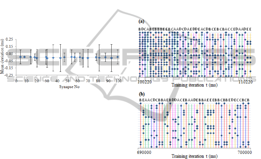
Figure 5: Mean deviation from pattern center in a single
"word" in L4 output (L4 to L4.1 synapses). Error bars
denominate standard deviations. Data retrieved from a
single experiment, the pattern repeated 521 times, only
consistent spikes that were repeated more than 80% of
times taken into account.
Fluctuations in patterns of "words" are caused by
variations of synaptic strength in L1.1 to L3
synapses and also depend on pre-existing value of
postsynaptic potential in L4 and L3 neurons. We did
not made analysis of which factor is dominant.
Another important detail is that due to presence of
errors in L1, not all spikes are equally consistent. In
Fig. 5 displayed L4 to L4.1 synapses that produced
consistent spikes at the range 83% to 100% of all
occurrences of the "word". In the rest of the
synapses spike occurred in less than 3% of the times.
Initially we failed to achieve L5 layer training in
these conditions within acceptable error rate.
Usually all neurons learned a single pattern or a few
at once. We solved this problem by introducing
stochastic threshold in L5 neurons: when neuron
reached its firing threshold, it didn't fire immediately
but with probability 0.8. This accelerated inhibition
from "lucky" competing neurons.
It must be noted, that attempts to apply stochastic
threshold in layer L1 only increased error rate.
4 RESULTS
We conducted a series of simulations of the entire
model in continuous mode. Also, because of high
computing cost of simulation of the entire network,
in order to estimate performance we conducted
experiments witch each of WTA sub networks
separately. Each of the simulations took 700000
iterations; first 100000 iterations were dedicated to
train L1 layer only with random “letters”. Typical
output from layer L5 at the beginning and at the end
of the training is displayed in Fig. 6.
Figure 6: Spike output from layer L5 at the beginning and
at the end of the training. Output from each of 20 L5
neurons aligned along vertical axis. Letters above pattern
denominate one of 5 sample "words" displayed at the time.
(a) Output at the beginning of the training. Even though
WTA network exposed to a very few appearances of each
sample of "word", consistent pattern started to emerge at
the very beginning of the training. (b) Output at the end of
the training.
4.1 Overall Performance of the Model
For estimation of the error rate, at the end of the
experiment we counted responses of individual
neurons relative to the sample occurrence times
during last 5000 iterations. For layer L1 we used
bias of 8 iterations latency for neuron response, and
bias of 16 iterations for layer L5. The sample to
which neuron was the most selective was assigned to
the neuron as a learned one. If neuron response
NEURAL PROCESSING OF LONG LASTING SEQUENCES OF TEMPORAL CODES - Model of Artificial Neural
Network based on a Spike Timing-dependant Learning Rule
201
count was less than a half of average sample, such
neuron was treated as non selective to any sample.
Each missed sample or neuron response out of the
biased sample window was treated as error. We did
not analyze the cases when neuron learned more
than one sample, instead treated responses to other
samples as errors.
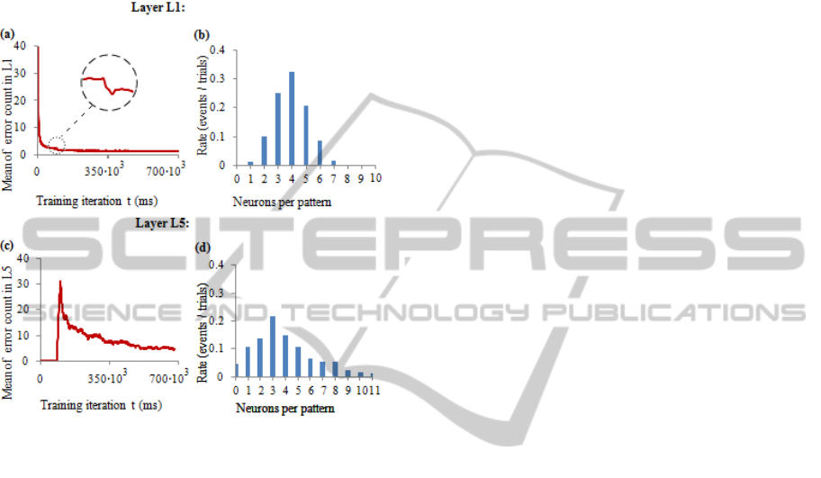
Figure 7: Mean error rate and selectivity distribution in
WTA layers L1 and L5. Data obtained from 100
experiments, each experiment made for 700000 iterations.
(a) Mean error rate in layer L1. Sample patterns were
regenerated for each experiment. Zoomed part of the
series indicates a drop of error rate after stochastic
appearance of one of the five samples (random letters)
were replaced by consistent sequences (random words).
(b) Distribution of the number of neurons selective to one
sample in layer L1. (c) Mean error rate in layer L5. Three
pre-recorded sample patterns of “words” were used in 100
experiments, each in 1/3 of experiments. (d) Distribution
of the number of neurons selective to one sample in layer
L5.
We conduced 100 of experiments to estimate
mean error rate for layers L1 and L5 separately.
Initial synaptic strengths were reset at each
experiment. Errors were counted in sliding 3000
iteration window for L1 and 18000 iterations for L5.
Window sizes were proportional to rate of samples 1
to 6: each word consisted of 5 letters plus 1 letter for
scant time. Window was moved by step of 1000
iterations (See Fig. 7). For layer L1 we generated
sample “letters” at each experiment, for layer L5 we
used recorded input from three different simulations
of the entire model. Therefore, our estimation of L5
error rate contains larger bias.
Layer L5 produced significantly larger error rate,
at the last 10000 iterations of experiments it reached
mean value of 4.514, while L1 produced only 1.207.
There is an interesting observation in layer L1
error rate: at the moment when random “letters” are
replaced by consistent sequences, we see modest but
steep drop in error rate (Fig. 7(a)). Most likely this is
caused by reduced rate of sequences of the same
"letter", what makes a trained neuron harder to fire
subsequently, because of previous hyperpolarization.
There were noticeable differences between layer
L1 and L5 in distribution of neurons selective to the
single pattern (See Fig. 7 (b) and (d)). Mean values
of the number of neurons per single sample were
quite close: 3.956 for L1 and 3.99 for L5, but
significantly different standard deviations: 1.24 for
L1 and 2.59 for L5. There were no any non-learned
samples in L1, but in L5 non-learned samples
occurred with the rate 0.046. Rate of neurons that
did not learn any pattern was significantly larger for
layer L1 and was 0.22, while in L5 it was 0.05. We
cannot tell which factor had the biggest influence to
this difference: different set of parameters, stochastic
threshold in L5, difference of input patterns, or it
was simply caused by biased measurements of layer
L5. It requires detailed theoretical study of limiting
and optimal parameters of STDP rules.
5 DISCUSSION
We demonstrated the model of an unsupervised
neural network that is capable of learning prolonged
combinations of spatiotemporal patterns of spikes in
continuous mode. In this way we demonstrated that
STDP learning rules alone can be applied to train
neural network to learn long lasting sequences
combined of short samples. Moreover, the model is
capable of memorizing and reproducing sequences
in which network input samples were displayed.
Reproduction of sequences can be achieved by
subsequently activating L2.1 neurons.
The fact, that memory of events in time can be
reproduced, implies that such memory could be
copied, transferred, compared etc. Also, it should be
relatively easy to extend our model enabling it to
learn combinations of "words", although that would
require additional, more complex modulation in
different time scales.
5.1 Biological Plausibility of the Model
The model itself and a range of parameters of
simulation are arbitrary and cannot be used as a
NCTA 2011 - International Conference on Neural Computation Theory and Applications
202

reference to a simulation of true biological process.
However, the model is based on known biological
processes, and presence of temporal coding is
supported by experimental evidence.
Since we designed our network to be as simple
as possible, there are, probably, many ways to
implement a neural network with similar or the same
features that would be more realistic in biological
sense or would have a better performance.
For an instance, for temporal modulation it
would be more realistic to use inhibitory neurons
instead of excitatory. There are experimental
evidences that gamma rhythm oscillations are
generated by inhibitory interneurons (Cardin et al.,
2009).
We used only the simplest closest-neighbor
approach to STDP learning rule. Other variations
could be considered for future experiments. For an
instance, a possible impact of triplet rule (Pfister and
Gerstner, 2006) should be taken into account.
5.2 Limitations of the Model and
Guidelines for Future Research
The model requires explicit timing for the
occurrence of training samples. In order to use our
model for real world data, timing of sensory input
must be aligned to activation periods of layer L2.
However, additional chains of modulation that
synchronizes sensory input with L2 layer activation
periods and/or vice versa should solve this problem.
Another obvious limitation of the model is a
"blind spot" at each memory read, however this
problem could be overcome by multiplying L1.1 to
L4 layers, in that way creating overlapping or sliding
memory window.
Simplistic structure of WTA networks used in
our model is disputable as well. With increase of
different sample count, intervals between the same
repeated sample would increase as well, that would
make learning harder and harder. Training individual
or groups of neurons one-by-one with a limited
number of samples would solve the problem and
boost the performance. However, how we would
implement this approach for a short temporal code in
rapidly changing environment is a question that we
cannot answer yet. Well known adaptive resonance
theory (ART) (Carpenter and Grossberg, 2009)
solves similar problem by introducing a self
organized network and a resonant state between
input and already learned data. However, the
achievement of resonance necessary for ART
requires a prolonged state of neural activity (rate
code) that is not the case of our model. Although,
various modifications of our model that would
introduce additional rate code are possible. This is
also a matter of future research.
The nonlinear nature of STDP and leaky
integrate-and-fire neuron makes the tuning of the
parameters of WTA networks a really challenging
task. We used genetic algorithm for this matter,
however, we cannot claim that we reached optimal
point of the model parameters. There is little known
of theoretical limits and optimal points of STDP
rule. Our next step will be detailed theoretical
research of STDP in the noisy environment from
perspective of the probability theory and statistics.
ACKNOWLEDGEMENTS
The author is thankful to Professor Sarunas Raudys
for useful suggestions and valuable discussion.
REFERENCES
Abbott L. F., Nelson S. B.. 2000. Synaptic plasticity:
taming the beast. Nat. Neurosci. 3:1178-1183
Abraham W. C. 2003. How long will long-term
potentiation last? Philos Trans R Soc Lond B Biol Sci
358: 735–744.
Bi, G. Q. and Poo, M. M. (1998). Synaptic modifications
in cultured Hippocampal neurons: dependence on
spike timing, synaptic strength, and postsynaptic cell
type. J Neurosci, 18:10464-72.
Bienenstock E. L., Cooper L. N., Munro P. W. (1982)
Theory for the development of neuron selectivity:
orientation specificity and binocular interaction in
visual cortex. J Neurosci 2:32–48.
Caporale N., Dan Y. (2008) Spike timing-dependent
plasticity: a Hebbian learning rule. Annu. Rev.
Neurosci.31:25–46.
Cardin, J. A. et al. (2009) Driving fast-spiking cells
induces gamma rhythm and controls sensory
responses. Nature 459, 663–667.
Carpenter G. A. and Grossberg, S. (2009). Adaptive
Resonance Theory. Technical Report CAS/CNS-TR-
2009-008.
Feldman D. E. (2000) Timing-based LTP and LTD at
vertical inputs to layer II/III pyramidal cells in rat
barrel cortex. Neuron 27:45–56.
Fellous J. M., Tiesinga P. H., Thomas P. J., Sejnowski T.
J. (2004) Discovering spike patterns in neuronal
responses. J Neurosci 24: 2989–3001.
Gerstner W., Kempter R., van Hemmen J. L., Wagner H.
(1996) A neuronal learning rule for sub-millisecond
temporal coding. Nature 383: 76–81.
Gerstner W., Kistler W. M. (2002) Spiking neuron
models. Cambridge: Cambridge UP.
NEURAL PROCESSING OF LONG LASTING SEQUENCES OF TEMPORAL CODES - Model of Artificial Neural
Network based on a Spike Timing-dependant Learning Rule
203

Guyonneau R., VanRullen R., Thorpe S. J. (2005)
Neurons tune to the earliest spikes through STDP.
Neural Comput 17: 859–879.
Hodgkin A. L., Huxley A. F (1952) A quantitative
description of membrane current and its application to
conduction and excitation in nerve, Journal
Physiology 117 500–544.
Kayser C., Montemurro M. A., Logothetis N. K., Panzeri
S. (2009) Spike-phase coding boosts and stabilizes
information carried by spatial and temporal spike
patterns. Neuron 61:597–608.
Masquelier, T., Guyonneau, R., Thorpe, S. J. (2008).
Spike timing dependent plasticity finds the start of
repeating patterns in continuous spike trains.
PLoSONE, 3(1), e1377.
Masquelier T., Guyonneau R., Thorpe S. J. (2009)
Competitive STDP-based spike pattern learning.
Neural Comput 21:1259–1276.
Pfister J-P, Gerstner W. (2006) Triplets of spikes in a
model of spike timing-dependent plasticity. J
Neurosci. 2006; 26:9673–9682.
Prut Y., Vaadia E., Bergman H., Haalman I., Slovin H., et
al. (1998) Spatiotemporal structure of cortical activity:
properties and behavioral relevance. J Neurophysiol
79: 2857–2874.
Song S., Miller K. D., Abbott L. F. (2000) Competitive
hebbian learning through spike-timing-dependent
synaptic plasticity. Nat Neurosci 3: 919–926.
VanRullen R., Thorpe S. J. (2001) Rate coding versus
temporal order coding: whatthe retinal ganglion cells
tell the visual cortex. Neural Comput 13: 1255–1283.
VanRullen R., Guyonneau R., Thorpe S. J. (2005) Spike
times make sense. Trends Neurosci. 28:1-4
Woodin M. A., Ganguly K., Poo M. M. 2003. Coincident
pre- and postsynaptic activity modifies GABAergic
synapses by postsynaptic changes in Cl- transporter
activity. Neuron 39:807–20
NCTA 2011 - International Conference on Neural Computation Theory and Applications
204
