
SEMI-SUPERVISED K-WAY SPECTRAL CLUSTERING
USING PAIRWISE CONSTRAINTS
Guillaume Wacquet, Pierre-Alexandre H´ebert,
´
Emilie Caillault Poisson and Denis Hamad
Universit´e Lille Nord de France, F-59000 Lille, France
Laboratoire d’Informatique, Signal et Image de la Cˆote d’Opale
ULCO, 50 rue Ferdinand Buisson, B.P. 699, F-62228 Calais Cedex, France
Keywords:
K-way spectral clustering, Semi-supervised classification, Pairwise constraints.
Abstract:
In this paper, we propose a semi-supervised spectral clustering method able to integrate some limited super-
visory information. This prior knowledge consists of pairwise constraints which indicate whether a pair of
objects belongs to a same cluster (Must-Link constraints) or not (Cannot-Link constraints). The spectral clus-
tering then aims at optimizing a cost function built as a classical Multiple Normalized Cut measure, modified
in order to penalize the non-respect of these constraints. We show the relevance of the proposed method with
an illustrative dataset and some UCI benchmarks, for which two-class and multi-class problems are dealt with.
In all examples, a comparison with other semi-supervised clustering algorithms using pairwise constraints is
proposed.
1 INTRODUCTION
The term ”spectral clustering” refers to a family of un-
supervised clustering algorithms. It is more and more
used thanks to its effectiveness and its simplicity of
implementation which comes down to the eigenvec-
tors extraction of a similarity matrix computed on the
dataset (Ng et al., 2002). Similarity matrix gathers
the complete information used by the method, telling
for each pair of instances how close they are. Con-
trary to some traditional clustering algorithms such as
K-means algorithm, the spectral clustering method al-
lows to deal with ”non-globular” clusters of points.
In recent years, methods incorporating prior
knowledge in their clustering process have emerged
as relevant and effective in several applications, such
as image segmentation (Meila and Shi, 2000), infor-
mation retrieval or document analysis (Han and Kam-
ber, 2006). The prior knowledge is generally provided
in two forms: class labels, and pairwise constraints.
Labelling data is a hard and long task. Pairwise con-
straints simply indicate if two instances must be in the
same cluster (Must-Link) or not (Cannot-Link). They
are easier to collect from experts than labels (Wagstaff
and Cardie, 2000). However, few works take an inter-
est in semi-supervised methods allowing to deal with
multiclass problems (K ≥ 2). Indeed, recent algo-
rithms mainly focus on two-class problems (K = 2).
In this paper, we propose a new algorithm able to
integrate constraints in the multiclass spectral clus-
tering process, using a penalty term in a way simi-
lar to the constrained Principal Components Analy-
sis (Zhang et al., 2007) used in dimension reduction.
The proposed algorithm aims at minimizing the MN-
Cut (Multiple Normalized Cut) criterion, while penal-
izing the non-respect of the given set of constraints.
Moreover, a convenient weight, easily interpretable,
is introduced in order to balance the MNCut and the
penalty term, i.e. the impact of the original struc-
ture of the data and the contribution of the constraints.
This method is compared with two recent algorithms,
and some proposed variants, on an artificial sample
and UCI datasets (http://archive.ics.uci.edu/ml/). The
results are finally presented, for different proportions
of known constrained pairs.
The paper is organized into three sections. The
first one is theoretical and presents the spectral clus-
tering algorithms and some semi-supervised methods
dealing with pairwise constraints. The second one
presents our semi-supervised K-way spectral cluster-
ing method. The last section assesses the perfor-
mances of our method and some recent algorithms
using synthetic dataset and public databases extracted
from UCI repository.
72
Wacquet G., Hébert P., Caillault Poisson É. and Hamad D..
SEMI-SUPERVISED K-WAY SPECTRAL CLUSTERING USING PAIRWISE CONSTRAINTS.
DOI: 10.5220/0003682500720081
In Proceedings of the International Conference on Neural Computation Theory and Applications (NCTA-2011), pages 72-81
ISBN: 978-989-8425-84-3
Copyright
c
2011 SCITEPRESS (Science and Technology Publications, Lda.)

2 STATE OF ARTS: K-WAY
SPECTRAL CLUSTERING,
PAIRWISE CONSTRAINTS
2.1 Graph Embedding and MNCut
Spectral clustering is generally considered as a clus-
tering method aiming at minimizing a Normalized Cut
criterion between K = 2 clusters (NCut), or a Multi-
ple Normalized Cut between K ≥ 2 clusters (MNCut)
(Meila and Shi, 2000)(Ng et al., 2002)(Shi and Ma-
lik, 2000). The first measure, NCut, assesses how
strongly a cluster of points (or vertices in a graph)
is linked to the other points, in relation to its own co-
hesion. The second one deals with multiple clusters
(K ≥2) and is set to the average of the NCut measures
over the whole clusters.
2.1.1 Notations
In order to prepare the NCut minimization problem
formulations, some notations are first introduced, us-
ing an usual graph formalism.
• Let X = {x
1
,...,x
i
,...,x
N
} be a set of N objects,
to be clustered;
• this set X is described by a weighted graph
G(V,E, S): V is the set of nodes corresponding
to the objects; E is the set of edges between the
nodes and S is a weights matrix whose elements
S
ij
= S
ji
≥ 0 tell how strongly related (or close)
objects x
i
and x
j
are;
• let D be the degree matrix of graph G, i.e. a di-
agonal matrix whose components are equal to the
degrees of the nodes: D
ii
=
∑
N
j=1
S
ij
;
• let C = {C
1
,...,C
K
} be a partitioning of X into
non-empty disjoint K subsets;
• each group C
k
is described by its volume
Vol(C
k
) =
∑
x
i
∈C
k
D
ii
and its “cohesion” degree
Cut(C
k
,C
k
) =
∑
x
i
∈C
k
∑
x
j
∈C
k
S
ij
;
• the Cut between two groups is defined by
Cut(C
k
,C
k
′
) =
∑
x
i
∈C
k
∑
x
j
∈C
k
′
S
ij
.
2.1.2 MNCut Minimisation as Eigenproblem
In a two-class problem, the Normalized Cut between
subsets C
1
and C
2
is defined as:
NCut(C
1
,C
2
) = Cut(C
1
,C
2
)
1
Vol(C
1
)
+
1
Vol(C
2
)
.
(1)
In a K-way clustering problem, NCut criterion is gen-
eralized by the Multiple Normalized Cut (MNCut):
MNCut(C) =
K
∑
k=1
Cut(C
k
,C\C
k
)
Vol(C
k
)
=
K
∑
k=1
1−
Cut(C
k
,C
k
)
Vol(C
k
)
(2)
Many authors of spectral clustering algorithms
have shown that the minimization of MNCut criterion
can be achieved by solving an eigenvalue system (or
generalized eigenvalue system). Their optimal clus-
tering processing can be resumed in three steps:
1. Computation and normalization of the similarity
matrix S. The result is generally a normalized
Laplacian matrix L.
2. Spectral Mapping. Some K vector solutions of an
eigenvalue system such as Lz
k
= λ
k
z
k
based on the
matrix issued from Step 1, are computed to form
the matrix Z = [z
1
,z
2
,... ,z
K
]. If the eigenvalues
are not distinct, the eigenvectors are chosen such
that z
T
i
Dz
j
= 0 for i 6= j. Z is then normalized
into a matrix U, whose each i-th row is used to
map object x
i
.
3. Partioning. A grouping algorithm like K-means
clusters the points in the spectral space, and as-
signs the obtained clusters to the corresponding
objects.
Now, some usual spectral algorithms are de-
scribed, in order to illustrate both paradoxal aspects:
the quasi-equivalence of their solutions, and the dif-
ference between the formalisms they adopt.
K = 2. Shi and Malik. In their paper (Shi and Ma-
lik, 2000), the authors define the indicator vector of
cluster C
1
as u ∈ {−1,1}
N
: u
i
= 1 ⇔ x
i
∈C
1
. NCut
criterion is then written as:
NCut(G,u) =
∑
x
i
>0,x
j
<0
−u
i
u
j
S
i, j
∑
x
i
>0
D
i,i
+
∑
x
i
<0,x
j
>0
−u
i
u
j
S
i, j
∑
x
i
<0
D
i,i
.
(3)
With variable change v = (1+ u) −b(1−u) with
b =
∑
x
i
>0
D
ii
/
∑
x
i
<0
D
ii
, infering both conditions v
i
∈
{1,−b} and v
T
D1 = 0, the above equation becomes a
Rayleigh quotient:
min
v
NCut(G, v) = min
v
v
T
(D−S)v
v
T
Dv
. (4)
By relaxing the constraints on indicator vector u
′
to take on real values, the minimization is obtained
by solving the generalized eigenvalue system: (D −
S)v = λDv that satisfies the constraint v
T
D1 = 0. By
setting z = D
1
2
v, a standard eigensystem, easier to
solve, is derived: D
−
1
2
(D−S)
−
1
2
z = λz.
SEMI-SUPERVISED K-WAY SPECTRAL CLUSTERING USING PAIRWISE CONSTRAINTS
73

So in Step 1, Shi and Malik compute the Laplacian
matrix L = D −S and its normalized variant L = I −
D
−
1
2
SD
−
1
2
.
In Step 2, they extract the second smallest eigen-
vector z of L, which is then transformed to approx-
imate the optimal vector indicator looked for: v =
D
−
1
2
z. First eigenvector z
0
, collinear to D
1
2
1, is left
in order to satisfy condition v
T
D1 = 0.
In Step 3, the objects are split into two clusters
based on the values of v (the optimal NCut splitting
value being looked for).
K = 2. Von Luxburg. In his tutorial (Luxburg,
2007), the author defines the indicator vector of clus-
ter C
1
as u ∈ {a, −a
−1
}
N
: u
i
= a ⇔ x
i
∈ C
1
, with
a =
q
Vol(C
2
)
Vol(C
1
)
. NCut criterion is then written as a
quadratic function of u:
NCut(G, u) =
1
2
∑
i, j
(u
i
−u
j
)
2
S
ij
=u
T
(D−S)u = u
T
Lu.
(5)
The problem solved is the same than Shi and Malik’s
one:
min
z
NCut(G, z) = min
z
z
T
Lz, s.t. z
T
z = 1, (6)
with exatly the same formal condition u
T
D1 = 0.
The same steps are then followed.
K >= 2. Shi and Malik, Von Luxburg. These au-
thors(Shi and Malik, 2000; Luxburg, 2007) general-
ize the NCut criterion to the Multiple-NCut (MNCut)
criterion, by proposing an average criterion:
MNCut(G,U) =
K
∑
k=1
NCut(G, u
k
),
whose K vectors u
k
, denote indicator vectors parti-
tioning X in K clusters.
Two authors((Meila and Shi, 2000; Luxburg,
2007)) propose to solve this problem, by considering:
u
k
∈ {0,
1
√
Vol(C
k
)
}
N
, and u
ik
=
1
√
Vol(C
k
)
⇔ x
i
∈ C
k
.
These indicator vectors are column-wise gathered in
matrix U.
They finally express their problem, in a way simi-
lar to case K = 2:
min
Z
MNCut(G,Z) = min
Z
K
∑
k=1
z
k
T
Lz
k
, s.t. z
k
T
z
k
= 1,
(7)
with additional formal condition U = D
−
1
2
Z:
U
T
DU = I. Let’s note that condition u
k
D1 will be
verified, although it is no more justified.
Consequently, the first K eigenvectors of L (i.e.
with the K smallest eigenvalues) minimize the cri-
terion and allow to estimate the K cluster indicator
vectors. In order to retrieve discrete cluster indica-
tor values, the eigenvector extraction is followed by a
K-means step on the row of U = D
−
1
2
Z.
Shi and Malik (Shi and Malik, 2000) describe the
same solution, but from a direct generalization from
case K = 2.
K >= 2. Ng et al.’s. The authors (Ng et al., 2002)
proposed an other algorithm based on Weiss (Weiss,
1999) and Meila and Shi (Meila and Shi, 2000) that
also solved the spectral problem (eq. 7), but without
formulating any optimization problem in terms of in-
dicator vectors.
They proposed to modify the initial similarity ma-
trix: S
ii
= 0, and to use the K highest eigenvectors
z
k
of L
Ng
= D
−
1
2
SD
−
1
2
, orthogonal to each others, to
map data. Let’s remark that these eigenvectors are the
K lowest eigenvectorsof I−L
Ng
= L. Then, instead of
computing a matrix U = D
−
1
2
Z from matrix Z stack-
ing the extracted eigenvectors, they rather project data
points in the spectral space on the unit-sphere, by nor-
malizing Z into U: U
ij
= Z
ij
/
q
∑
j
Z
2
ij
.
Step 3 is K-means too, initialized by points at most
orthogonal.
Despite the diversity of the formalisms used to
define the indicator vectors, all these authors finally
solve the same objective function (eq. 7), which in-
volves the same normalized Laplacian matrix L.
2.2 Spectral Clustering Methods using
Pairwise Constraints
2.2.1 Pairwise Constraints Information
We now focus on additional knowledge, formalized
as pairwise constraints. The set of objects X and its
similarity matrix S is now completed with the follow-
ing two sets of pairs of objects (Wagstaff and Cardie,
2000):
• pairs of points that must belong to different clus-
ters: {x
i
,x
j
}∈C L , with {x
i
,x
j
}⊆X , the Cannot-
Link set of pairs;
• pairs of points that must belong to the same clus-
ter: {x
i
,x
j
} ∈ M L , with {x
i
,x
j
} ⊆ X , the Must-
Link set of pairs.
NCTA 2011 - International Conference on Neural Computation Theory and Applications
74

Spectral clustering methods integrating this type of
information has previously been proposed, first by
Kamvar et al. (Kamvar et al., 2003), and more re-
cently by Wang and Davidson (Wang and Davidson,
2010). Both methods are now presented, while hight-
lighting some of their weakness.
2.2.2 Spectral Learning Method
In (Kamvaret al., 2003), the constrained spectral clus-
tering method described is built as a basic spectral
clustering method, in which two steps are modified:
• the similarity matrix S, built by applying a gaus-
sian kernel on a set of N points describing the ob-
jects in X , is modified in the following way: for
each pair {x
i
,x
j
} ∈ M L , elements S
ij
= S
ji
are
set to 1; and for each pair {x
i
,x
j
}∈ C L , elements
S
ij
= S
ji
are set to 0;
• then, similarity matrix S is not normalized as in
the MNCut-graph paradigm, but in a normalized
additive way: (S+ d
max
I −D)/d
max
, with d
max
the
maximal rowsum of S; the obtained matrix is a
symmetric Markov transition probabilities matrix;
the authors underline that must-linked pairs have
a higher mutual transition value than other pairs;
eigenvectors are then extracted from this normal-
ized S, and their rows are unit-length normalized.
The main weakness of this variant is that must-
linked (respectively, cannot-linked)similarities are ar-
bitrarly set to their maximal (r., minimal) theoriti-
cal values: 1 and 0. About the maximal value, and
even for the minimal value (although the paper is
focused on Markov’s probability matrix formalism),
this choice may be discussed: greater or smaller val-
ues could have been prefered. With such a priori val-
ues, it’s difficult to know if the constraint on pairs of
points is excessive, weak, or well balanced.
2.2.3 Flexible Constrained Spectral Clustering
Method
In their paper (Wang and Davidson, 2010), Wang and
Davidson express their constrained spectral cluster-
ing problem, as a constrained optimization problem,
which is solved by an eigenvector extraction. Their
approach is consequently less empirical than the pre-
vious one, and it gives an answer to the problem of
tuning the strength of the constraints.
The semi-supervised spectral clustering problem
is detailed with K = 2. The indicator vector looked
for is denoted u ∈ { −1,+1}
N
, and the satisfaction of
pairwise constraints is measured thanks to a matrix Q:
Q
ij
= Q
ji
=
−1 if {x
i
,x
j
} ∈ C L ,
+1 if {x
i
,x
j
} ∈ M L ,
0 else.
(8)
With such a Q matrix, the measure u
T
Qu increases
with the number of satisfied constraints.
The problem is then formulated as a constrained
optimization problem, letting z = D
1
2
u and Q =
D
−
1
2
QD
−
1
2
:
min
z
z
T
Lz,
s.t. z
T
Qz ≥α, z
T
z = Vol(G), z 6= D
1
2
1.
(9)
The first constraint lower-bounds the satisfaction
of constraints, the second one normalizes the indica-
tor vector, and the last one is intented to avoid the triv-
ial solution of spectral clustering (i.e. the “constant”
indicator vector).
The problem is finally solved using Lagrange mul-
tipliers, but the infinite set of solutions has to be re-
duced by constraining this multipliers.
A feasible set of eigenvectors z, is then set as the
solutions of the following generalized eigenproblem
whose eigenvalues λ are strictly positive (because of
the constraints satisfaction):
Lz = λ(Q−
θ
Vol(G)
I)z. (10)
And the optimal z is then selected as the one min-
imizing the MNCut measure z
T
Lz, while differing
from the trivial solution D
1
2
1. Final indicator vector
solution u is then obtained from the usual: u = D
−
1
2
z.
Parameter θ is used to weight the constraints im-
pact: θ < λ
max
Vol(G), with λ
max
the largest eigen-
value of Q. The authors propose the following a pri-
ori value:
θ = λ
max
×Vol(G) ×
0.5+ 0.4 ×
# Constraints
N
2
.
As shown in their paper (Wang and Davidson,
2010) in case K = 2, this algorithm outperforms Kam-
var’s method, which directly modifies the similarity
matrix using 0 and 1 values.
In case K > 2, although the authors generalize the
method by selecting not only the first, but the top-
K generalized eigenvectors corresponding to the pos-
itive eigenvalues, we generally observe lower perfor-
mances on UCI benchmarks, sometimes even lower
than Kamvar’s method ones.
As a possible explanation of these differences, we
remark that the K-dimensional spectral subspace is
not built as in the original spectral clustering method:
SEMI-SUPERVISED K-WAY SPECTRAL CLUSTERING USING PAIRWISE CONSTRAINTS
75

0 20 40 60 80 100
0.6
0.65
0.7
0.75
0.8
0.85
0.9
0.95
1
% known labels
Rand Index
FCSC-θSP
FCSC
SL-MOD
SL
(a) Glass (K = 2).
0 20 40 60 80 100
0.5
0.55
0.6
0.65
0.7
0.75
0.8
0.85
0.9
0.95
1
% known labels
Rand Index
FCSC-θSP
FCSC
SL-
¯
L
SL
(b) Wine (K = 3).
Figure 1: Rand Index on two UCI datasets, functions of the
percentage of known labels. (FCSC-θSP: modified version
of FCSC, FCSC: original version of FCSC, SL-L: modified
version of SL, SL: original version of SL).
in particular, properties u
T
k
D1 = 0 and u
T
k
Du
k
′
= 0 are
generally not satisfied. Although they are not always
constrained in the original MNCut minimization prob-
lem (it depends on the formalism used), they could
favour better clustering.
Let’s finally remark that, on contrary to Von
Luxburg’s approach, the conditions verified by the
eigenvectors are not justified by the formalism used
(u
k
∈ {−1,1}
N
): neither equations z
T
k
Lz
k
′
= 0 ⇔k 6=
k
′
and z
T
k
(Q−
θ
Vol(G)
)z
k
⇔k 6= k
′
, nor equation u
T
k
D1.
3 SEMI-SUPERVISED K-WAY
SPECTRAL CLUSTERING
ALGORITHM
Our problem formulation consists in a MNCut prob-
lem, where the objective function is modified, in such
a way to penalize the non-respect of constraints. Un-
like to FCSC method, the spectral subspace is ob-
tained from a basic spectral clustering algorithm.
3.1 Penalty Cost
This penalty cost could be expressed on the indicator
vector u
k
. First, we should have to decide which bi-
nary domain of values {a, b} to use, such that u
k
∈
{a,b}
N
. But we prefer here to consider that this do-
main choice does not matter a lot: all the spectral
clustering methods presented in Section 2 including
Wang’s one, whatever this domain is, finally define
the spectral subspace from the top-K eigenvectors z
k
from Laplacian matrix L = D
−
1
2
SD
−
1
2
, i.e. the ones
minimizing L = I −D
−
1
2
SD
−
1
2
. The penalty cost will
then depend on these eigenvectors z
k
, stacked in ma-
trix Z.
Then, previous methods post-transform these vec-
tors, either by a D
−
1
2
pre-multiplication, or by a pro-
jection on the unit-sphere. We consider here this last
choice, as in different previously presented methods
(Ng et al., 2002)(Kamvar et al., 2003).
Because of this final projection, we decide to
make the penalty cost depend on the angles be-
tween spectral projections given by the K eigenvec-
tors. Penalty term PC is defined by dot products be-
tween constrained points, considering that this mea-
sure suits well to the alteration of angles:
PC = PC(C L ,M L ,α,β,Z)
=
−α
|C L |
∑
{x
i
,x
j
}∈C L
K
∑
k=1
z
ik
.z
jk
+
β
|M L |
∑
{x
i
,x
j
}∈M L
K
∑
k=1
z
ik
.z
jk
=
K
∑
k=1
−
α
|C L |
∑
{x
i
,x
j
}∈C L
z
ik
.z
jk
+
β
|M L |
∑
{x
i
,x
j
}∈M L
z
ik
.z
jk
.
Weights α and β are used to balance the con-
tributions of the must-linked and cannot-linked con-
straints. Zhang et al. incorporate a quite similar
Pairwise-Constraints penalty cost in a PCA method
(Zhang et al., 2007), but with an Euclidean distance
measure. As they do, we now express penalty cost PC
as a matrix product, using a more general cost matrix
Q than Wang’s one:
Q
ij
= Q
ji
=
−
α
|C L |
if {x
i
,x
j
}∈ C L ,
+
β
|M L |
if {x
i
,x
j
}∈ M L ,
0 else.
(11)
PC term is then written in the following way:
PC =
1
2
∑
i, j
K
∑
k=1
z
ik
z
jk
Q
ij
=
K
∑
k=1
z
T
k
Qz
k
. (12)
3.2 Penalized MNCut Cost Function
This penalizing term is now combined to the MNCut
criterion, so as to build a pairwise constrained spectral
clustering optimization problem:
J = J(G,C L ,M L ,Z)
= MNCut(G,Z) + PC(C L ,M L ,α,β,Z).
(13)
Minimizing this objective function allows to char-
acterize a spectral projection reflecting both the origi-
nal structure of data and the constraints proposed. We
now want to revealthe criterion PC as a Rayleigh quo-
tient, in order to set our problem as an eigenproblem.
MNCut and PC costs are now introduced in Equa-
tion 13:
J =
K
∑
k=1
z
T
k
Lz
k
+
K
∑
k=1
z
T
k
Qz
k
=
K
∑
k=1
z
T
k
(L+ Q)z
k
. (14)
NCTA 2011 - International Conference on Neural Computation Theory and Applications
76

The penalized optimization problem can then set
as:
min
Z
K
∑
k=1
z
T
k
(L+ Q)z
k
, s.t. z
k
T
z
k
= 1. (15)
This problem is clearly related to the basic spec-
tral clustering’s one Equation 7, except that the nor-
malized Laplacian matrix L is penalized by matrix Q
carrying the set of pairwise constraints.
3.3 Setting the Balance between the
Two Parts of Criterion J
Considering that a ML information has the same im-
portance as a CL information, and that the necessary
strength to force them may be equal, we set α = β;
in the following part, these weights will be tuned by
variable γ.
In addition, we propose a normalization making J
easier to interpret. The MNCut expression z
T
k
Lz
k
be-
longing to [0, 1] and the penalty one z
T
k
Qz
k
belonging
to [λ
Qmin
,λ
Qmax
], we propose to normalize matrix Q
using its minimal and maximal eigenvalues λ
Qmin
and
λ
Qmax
: Q =
Q−λ
Qmin
λ
Qmax
−λ
Qmin
.
Thanks to balancing term γ, criterion J now be-
longs to [0,1], and the final problem is set as:
min
Z
K
∑
k=1
((1−γ).z
k
T
Lz
k
+ γ.z
k
T
Qz
k
),
s.t. z
k
T
z
k
= 1.
(16)
3.4 “Mono-cluster” Solution u
0
= D
1
2
1
Because of the penalty term used, this vector is not
solution of our optimization problem for most Q ma-
trix, on contrary to basic spectral clustering’s one or
even to Wang’s constrained spectral clustering prob-
lem. This can be seen as a weakness, because it’s
make mono-cluster vectors more difficult to recog-
nize and to reject: in basic spectral clustering, all the
eigenvectors orthogonal to z
0
(the smallest eigenvec-
tor of L) are necessarily valid solutions.
To overcome this problem, a simple Euclidean
distance can be used instead of the dot product penalty
measure: matrix Q would then be modified by the
substraction of a diagonal matrix R composed of its
rowsums: R
ii
=
∑
j
Q
ij
. With this penalty measure
used on U = D
−
1
2
Z rather than on Z, mono-cluster
vector u
0
becomes a solution of the obtained eigen-
system, quite similar to the one proposed; so it can be
easily rejected. But in practice, the obtained results on
all the benchmarks tested were less performant; that
is why this solution was left.
In case K = 2, we then decide to reject the mono-
cluster solution obtained from vectors u containing
only positive (or negative) values.
In case K > 2, we maintain the usage of K eigen-
vectors, considering that this mono-cluster vector has
high chance to take part in the subspace building. All
the experiments made did not appear to be penalized
by this point, as it will be shown in the next section.
The algorithm in its K-way variant is resumed be-
low (cf. Algorithm 1).
Algorithm 1: Semi-Supervised K-way Spectral Clustering.
Spectral projection step
1. For a given data matrix X ∈ ℜ
N×P
, with N points
described in a P-features space, compute a sim-
ilarity matrix S between these points ; for exam-
ple: S
ij
= e
−
d
2
(x
i
,x
j
)
2σ
2
, with σ a scale parameter, and
d a distance measure.
2. Set S
ii
= 0.
3. Compute the constraints weighting matrix Q:
Q
ij
=
−
1
|C L |
if {x
i
,x
j
} ∈ C L ,
+
1
|M L |
if {x
i
,x
j
} ∈ M L ,
0 else.
4. Compute the minimum and maximum eigenval-
ues (denoted λ
Qmin
and λ
Qmax
) of Q.
5. Compute the constraints weighting matrix Q:
Q =
Q−λ
Qmin
λ
Qmax
−λ
Qmin
6. Compute the degree diagonal matrix D ∈ ℜ
N×N
:
D
ii
=
∑
j
S
ij
.
7. Compute the normalized Laplacian matrix: L =
I −D
−
1
2
SD
−
1
2
.
8. Find, the K lowest eigenvectors {z
1
,... , z
K
} of
matrix:
(1−γ)L+ γQ,
and form the matrix Z = [z
1
,... ,z
K
] ∈ ℜ
N×K
.
9. Normalize the rows of Z to be unit-lengthed (pro-
jection on the unit-sphere).
Spectral clustering step
1. Apply a K-means clustering on the data matrix Z.
2. Cluster each point of X as its corresponding point
in Z was clustered.
SEMI-SUPERVISED K-WAY SPECTRAL CLUSTERING USING PAIRWISE CONSTRAINTS
77

4 EXPERIMENTAL RESULTS
In this section, our Semi-Supervised Spectral Clus-
tering method (denoted SSSC) is applied first on
some illustrative synthetic examples, then on public
benchmarks belonging to the UCI repository. For
each dataset, some pairwise constraints are generated
from the known labels, and results are analyzed using
objective evaluation measures like MNCut, satisfied
constraints rates, or Rand Index. These results are
then compared with outputs of a set of similar meth-
ods (like Kamvar’s and Davidson’s ones).
4.1 Algorithms for Comparison
For all experiments, the proposed algorithm is com-
pared with the following seven clustering methods:
• SC: the basic Spectral Clustering Ng’s algorithm
(cf. 2.1.2), as a control reference unsupervised
method, in order to assess the impact of the added
pairwise constraints on the initial clustering;
• SL: the original semi-supervised Spectral Learn-
ing algorithm introduced in Section 2.2.2;
• SL-L: a modified version of the SL algo-
rithm, whose Laplacian matrix is replaced by the
one used in our SSSC method (i.e. L = I −
D
−
1
2
SD
−
1
2
);
• FCSC: the original Flexible Constrained Spectral
Clustering method introduced in Section 2.2.3,
weighted by the value θ obtained from the rule
given by the authors;
• FCSC-θ: a variant of FCSC, where the
weight θ is a posteriori choosed in the range
(λ
min
Vol(G),λ
max
Vol(G)) introduced by the au-
thors, using an exhaustive search;
• FCSC-θSP: a variant of FCSC-θ, which consists
in incorporating the projection on the unit-sphere
step;
• FCSC-θ
2
SP: a variant of FCSC-θSP, where pa-
rameter θ is looked inside a range larger than the
one proposed by the authors.
In order to facilitate the comparison of the meth-
ods, without promoting our SSSC method, some ho-
mogenisations were done. Except for methods FCSC
and FCSC-θ, the projection step on the unit-sphere is
applied. The integration of this step in the algorithms
facilitates the comparison and allows to not promote
our SSSC method.
In all FCSC variants except the original one, the
weighting matrix used for experiments is the one de-
fined in Algorithm1. The weights of each kind of con-
straints are then similar and depend on the number of
contraints defined.
For SSSC and FCSC variants (except the original),
the weight of the penalty term θ or γ is a posteriori
optimized, by discretizing their definition interval into
100 equidistant values, and choosing the one which
maximizes the criterion:
E = (1−MNCut) + M L
satisfied
+ C L
satisfied
, (17)
where M L
satisfied
and C L
satisfied
are the respective
rates of satisfied M L and C L constraints.
For FCSC-θ and FCSC-θSP, the optimal θ in
searched in the range [λ
min
Vol(G),λ
max
Vol(G)]. The
authors show that this range is sufficient to assure
the existence of K vectors satisfying the constraint of
their optimization problem; moreover, it contains the
values in which the constraints are at most satisfied
(Wang and Davidson, 2010).
For FCSC-θ
2
SP, we decide to enlarge the range
used: [−100 × max(|λ
min
|,|λ
max
|) × vol(G),λ
max
].
The lower bound is an empirical value choosed in or-
der to make their constraint problem converge to the
unconstrained spectral clustering method, like in our
method.
4.2 Illustrative Example
To study the effect of constraints in clustering, we
propose to use pairwise constraints in a multiclass
problem.
The dataset is composed of 400 data samples
drawn from a mixture of five bivariate Gaussian dis-
tributions, as shown in Figure 2(a). The proportion of
each Gaussian distribution is set to
1
5
. In this case, the
desired number of clusters K is set to 4.
Three pairwise informations are considered: two
ML constraints between data points from different
clusters, and one CL constraint between two data
points from the same Gaussian cluster (cf. Figure
2(a)). These pairwise constraints were deliberately
chosen so as to make the expected clustering differ
from the natural minimal cut obtained by the Spectral
Clustering algorithm (SC) (i.e. we try to break the
natural cut of the dataset).
For this example, the similarity matrix is built
from a Gaussian kernel with a scale parameter σ set
to 1, and with d set to the Euclidean distance.
Figure 2 shows the clusterings resulted for the
eight methods tested. Here, FCSC clustering is not
shown because its optimization problem can not be
solved for the given value of θ; in fact, the proposed
rule is clearly not suitable to case K > 2.
While all others methods fail to break the natural
cut, the proposed SSSC, FCSC-θSP and FCSC-θ
2
SP
NCTA 2011 - International Conference on Neural Computation Theory and Applications
78
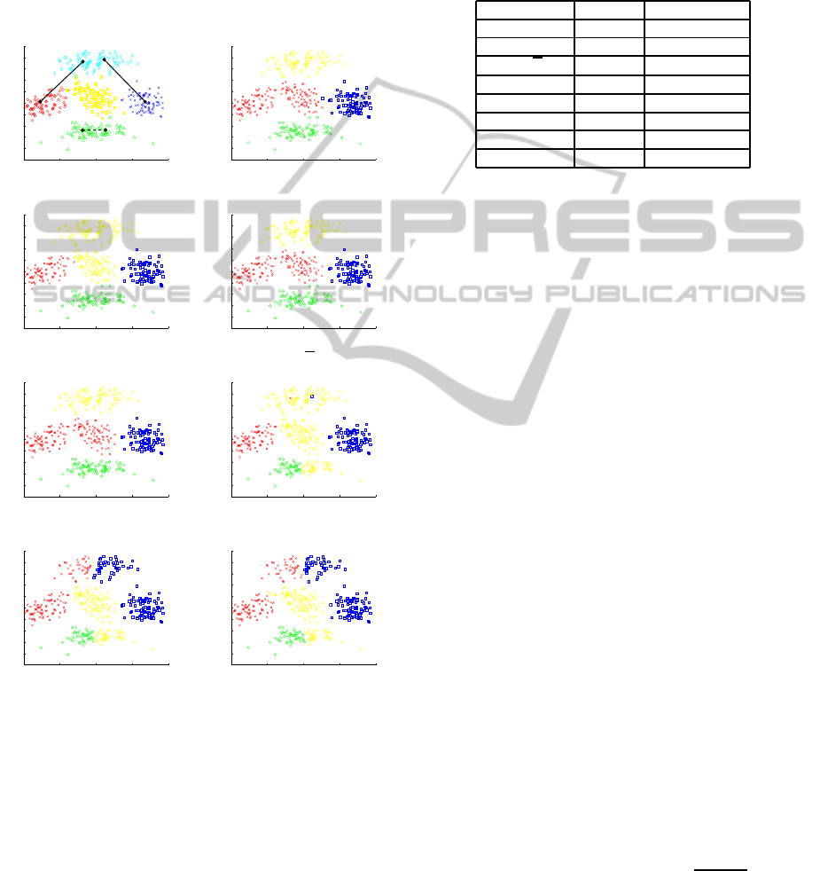
succeed in imposing the three constraints, as shown in
Figure 2(f), (g) and (h). The combination of the three
pairwise constraints succeeds in affecting the cluster-
ing, even with a “non-natural”CL constraint.
In order to complete the analyse of these cluster-
ing results, some performance indicators such as MN-
Cut values and the total proportion of satisfied con-
straints (ML and CL) are shown in Table 1.
−5 0 5 10 15
4
6
8
10
12
14
16
18
20
22
24
−5 0 5 10 15
4
6
8
10
12
14
16
18
20
22
24
Original data. SC.
−5 0 5 10 15
4
6
8
10
12
14
16
18
20
22
24
−5 0 5 10 15
4
6
8
10
12
14
16
18
20
22
24
SL. SL-L.
−5 0 5 10 15
4
6
8
10
12
14
16
18
20
22
24
−5 0 5 10 15
4
6
8
10
12
14
16
18
20
22
24
FCSC-θ. FCSC-θSP.
−5 0 5 10 15
4
6
8
10
12
14
16
18
20
22
24
−5 0 5 10 15
4
6
8
10
12
14
16
18
20
22
24
FCSC-θ
2
SP. SSSC.
Figure 2: Clustering results on Bivariate Gaussian clusters
with 2 ML and 1 CL constraints.
Worst MNCUT values are obtained from SSSC,
FCSC-θSP and FCSC-θ
2
SP methods, but they are the
only ones which satisfy the pairwise constraints, nec-
essarily at the expense of MNCut. The MNCut for
SSSC is smaller than for FCSC-θSP and FCSC-θ
2
SP,
as shown in Table 1.
In this case, FCSC-θSP does not appear very
performant: despite its high rate of satisfied con-
straints, it tends to isolate the data points linked
by these pairwise constraints, in contrary of SSSC
and FCSC-θ
2
SP. Weights of proposed interval
[λ
min
Vol(G),λ
max
Vol(G)] appear too high in this
case.
Table 1: MNCut values and percentage of satisfied con-
straints, for the different methods with 2 ML and 1 CL con-
straints.
Methods MNCut %(ML +CL)
SC 0.004 0.0
SL 0.0151 0.0
SL-L 0.013 0.0
FCSC / /
FCSC-θ 0.030 0.0
FCSC-θSP 0.048 100.0
FCSC-θ
2
SP 0.042 100.0
SSSC 0.031 100.0
This experiment shows that the introduction of
prior knowledge is well managed by SSSC method
and FCSC modified method (variant FCSC-θ
2
SP).
The comparison with the basic Spectral Clustering
method shows that supplying prior information, in the
form of pairwise constraints, allows to improve the
clustering accuracy.
Moreover, in this example, the proposed SSSC
method succeeds in conjointly satisfying both con-
straints and minimal MNCut score, in a more efficient
way than all other algorithms.
4.3 Application to UCI Datasets
In this section, our Semi-Supervised K-way Spectral
Clustering method is applied to some datasets well-
known in the classification world (UCI datasets). For
each example, some given proportions of objets are
randomly selected, so as to build sets of labelled ob-
jects. Then, they are used to deduce both C L and
M L constraints sets. For each percentage tested, we
enlarge the previous sets of constraints with new in-
formations. The quality of the clusterings obtained is
measured by the Rand index, which reflects the simi-
larity between the complete known partition (ground
truth) and the one obtained, depending on the num-
ber of pairs of points classified similarly in the two
partitions (Wagstaff and Cardie, 2000). The perfor-
mance scores are averaged over 10 repetitions of the
constraints generation process.
Table 2 shows the six datasets used. The data
preprocessing is described in (Wang and Davidson,
2010). For each example, the similarity matrix is built
using a Gaussian kernel: S
ij
= exp(−
||x
i
−x
j
||
2
2σ
2
) where
σ is the scale parameter equal to the mean of the vari-
ances of features.
Figure 3 shows the performance measures of all
the methods applied on these UCI datasets, in terms
SEMI-SUPERVISED K-WAY SPECTRAL CLUSTERING USING PAIRWISE CONSTRAINTS
79

0 20 40 60 80 100
0.6
0.65
0.7
0.75
0.8
0.85
0.9
0.95
1
% known labels
Rand Index
FCSC-θSP
FCSC-θ
FCSC
FCSC-θ
2
SP
SL-
¯
L
SL
SSSC
0 20 40 60 80 100
0.5
0.55
0.6
0.65
0.7
0.75
0.8
0.85
0.9
0.95
1
% known labels
Rand Index
0 20 40 60 80 100
0.5
0.55
0.6
0.65
0.7
0.75
0.8
0.85
0.9
0.95
1
% known labels
Rand Index
Glass1 (K = 2). Hepatitis (K = 2). Ionosphere (K = 2).
0 20 40 60 80 100
0.7
0.75
0.8
0.85
0.9
0.95
1
% known labels
Rand Index
0 20 40 60 80 100
0.6
0.65
0.7
0.75
0.8
0.85
0.9
0.95
1
% known labels
Rand Index
0 20 40 60 80 100
0.3
0.4
0.5
0.6
0.7
0.8
0.9
1
% known labels
Rand Index
Wine (K = 3). Dermatology (K = 6). Glass2 (K = 6).
Figure 3: Rand Index (mean, maximum and minimum), functions of the percentage of known labels, on UCI datasets.
Table 2: UCI datasets.
Nb. Ob-
jects
Nb. Fea-
tures
Nb.
Classes
Glass1 214 9 2
Hepatitis 80 19 2
Ionosphere 351 34 2
Wine 178 13 3
Dermatology 366 34 6
Glass2 214 9 6
of Rand index, i.e. the rate of pairwise relations equal
to the real ones. As it can be observed:
• Globally, methods like SSSC and some FCSC
variants achieve to significantly improves the ba-
sic spectral clustering (corresponding to abscissa
0). Increasing the number of constraints globally
improves the performances, and this increase is
faster between abscissa 0% and 5%. This means
that best methods are able to improve the cluster-
ing with small amongs of pairwise constraints.
• For K = 2, the best results are obtained from
methods SSSC and all FCSC variants except
FCSC-θ
2
SP: their Rand indexes are the highest
and the more stable: they do not decrease with
the number of constraints added.
SL-L and FCSC-θ
2
SP show quite lower perfor-
mances. The superiority of FCSC over FCSC-
θ
2
SP may be explained by the fact that FCSC-
θ
2
SP searches the optimal value of θ in a larger
range than FCSC-θSP, but with the same dis-
cretization step (100 values): some interesting
values may consequently be omitted. This tends
to show that the choice of this parameter is not
so obvious in FCSC method. SL-L becomes in-
teresting, only with high numbers of constraints:
weigths 0 and 1 seem too low (in absolute value)
to impact the clustering.
Then SL gives the lowest Rand indexes: the
Laplacian used does not achieve to minimize the
NCut measure.
• For K > 2, SSSC gets better performances than all
others methods. FCSC-θ
2
SP and SL-L give sec-
ond best results. FCSC-θSP’s ones are lower (the
range of θ being too small). Then the methods
FCSC-θ and SL give very low Rand indexes: both
weigths and projection step are required to assure
good performances. FCSC original method does
not appear, because the constrained problem is not
solved with the proposed θ value.
Table 3 shows some performance indicators of the
different methods applied on a specific example, Der-
matology, whose number of clusters K is set to 6. In
each category, percentage of known labels by perfor-
mance indicator, the best result is printed in bold type.
The proposed method thus appears to be very
competitive versus the other methods tested. Indeed,
for these datasets, SSSC method frequently reaches
the highest rates of satisfied constraints (over 99% for
each case), while keeping a satisfactory MNCut value
for each percentage of known labels (almost always
NCTA 2011 - International Conference on Neural Computation Theory and Applications
80

Table 3: Evaluation measures on ”Dermatology” dataset
(K = 6) with different numbers of constraints.
%
known
labels
Methods %
ML
% CL % To-
tal
MNCut Rand
Index
0 SL / / / 0.245 0.805
SL-L / / / 0.013 0.827
FCSC / / / 0.011 0.814
FCSC-θ / / / 0.011 0.814
FCSC-θSP / / / 0.013 0.827
FCSC-
θ
2
SP
/ / / 0.013 0.827
SSSC / / / 0.013 0.827
2 SL 100.0 87.1 93.5 0.251 0.808
SL-L 100.0 94.1 97.1 0.059 0.850
FCSC / / / / /
FCSC-θ 48.8 70.7 59.7 0.085 0.800
FCSC-θSP 37.4 80.7 59.1 0.109 0.869
FCSC-
θ
2
SP
100.0 100.0 100.0 0.036 0.894
SSSC 100.0 99.7 99.9 0.013 0.880
5 SL 100.0 84.1 92.1 0.273 0.806
SL-L 100.0 95.7 97.9 0.038 0.900
FCSC / / / / /
FCSC-θ 65.0 77.6 71.3 0.102 0.799
FCSC-θSP 62.8 92.3 77.6 0.139 0.890
FCSC-
θ
2
SP
96.7 95.0 95.9 0.040 0.909
SSSC 100.0 98.4 99.2 0.018 0.914
100 SL 100.0 100.0 100.0 0.063 1.000
SL-L 100.0 100.0 100.0 0.063 1.000
FCSC / / / / /
FCSC-θ 75.8 70.3 73.0 0.334 0.714
FCSC-θSP 72.5 87.7 80.1 0.095 0.847
FCSC-
θ
2
SP
87.6 93.9 90.8 0.037 0.927
SSSC 100.0 100.0 100.0 0.045 1.000
lower than other methods).
For example, for a small percentage of known la-
bels (5%), the total proportion of satisfied constraints
(ML and CL) for SSSC is better than for the oth-
ers methods (99.2%) and the MNCut value is small
(0.018). Moreover, this value is coherent with the one
obtained for the basic spectral clustering (correspond-
ing to 0% of known labels and equal to 0.013) and is
smaller than for SL, SL-L and the four FCSC meth-
ods. Best Rand index is achieved too (0.914): final
result for SSSC is then closer to the optimal cluster-
ing than other methods.
For a lower percentage (2%), SSSC method sat-
isfies not exactly all constraints (99.9%), contrary to
FCSC-θ
2
SP. But its MNCut is the lowest (0.13 versus
0.36).
5 CONCLUSIONS
In this paper, we proposed a new efficient K-way
spectral clustering algorithm, using Cannot-Link and
Must-Link as semi-supervised information. Like in
its unsupervised version, the clustering problem is set
as an optimization problem, consisting in minimiz-
ing an objective function proportional to the Multiple
Normalized Cut measure. This measure is here bal-
anced by a weighted penalty term assessing the non-
satisfaction of the given constraints.
Some comparisons with similar methods have
been carried on synthetic samples and some UCI
benchmarks. Different variants of the compared
methods have been proposed, in order to make the
methods more comparable, so as to get fair conclu-
sions. In all cases, the results illustrated that the most
performing methods, ours and the modified Wang’s
algorithms, are able to rapidly adjust the initial clus-
tering to a more convenient one, satisfying the given
constraints, even with quite low numbers of con-
straints. Our method seems to be part of this head
group of methods, its clusterings often achieving the
lowest MNCut values, and the highest satisfied con-
straints rates in the two-class and multi-class cases.
These experiments highlighted the importance of two
steps in this kind of semi-supervised spectral cluster-
ing methods: first, the usual projection step of basic
spectral clustering appears as crucial; then, a lot of
efforts have to be done to tune the constraints weight.
REFERENCES
Han, J. and Kamber, M. (2006). Data Mining: Concepts
and Techniques. Morgan Kaufmann Publishers.
Kamvar, S., Klein, D., and Manning, C. (2003). Spectral
learning. In IJCAI, International Joint Conference on
Artificial Intelligence, pages 561–566.
Luxburg, U. (2007). A tutorial on spectral clustering. In
Statistics and Computing, pages 395–416.
Meila, M. and Shi, J. (2000). Learning segmentation by
random walks. In NIPS12, Neural Information Pro-
cessing Systems, pages 873–879.
Ng, A., Jordan, M., and Weiss, Y. (2002). On spectral clus-
tering: Analysis and an algorithm. In NIPS14, Neural
Information Processing Systems, pages 849–856.
Shi, J. and Malik, J. (2000). Normalized cuts and image seg-
mentation. In PAMI, Transactions on Pattern Analysis
and Machine Intelligence, pages 888–905.
Wagstaff, K. and Cardie, C. (2000). Clustering with
instance-level constraints. In ICML, International
Conference on Machine Learning, pages 1103–1110.
Wang, X. and Davidson, I. (2010). Flexible constrained
spectral clustering. In KDD, International Conference
on Knowledge Discovery and Data Mining, pages
563–572.
Weiss, Y. (1999). Segmentation using eigenvectors: an
unifying view. In IEEE, International Conference on
Computer Vision, pages 975–982.
Zhang, D., Zhou, Z., and Chen, S. (2007). Semi-supervised
dimensionality reduction. In SIAM, 7th International
Conference on Data Mining, pages 629–634.
SEMI-SUPERVISED K-WAY SPECTRAL CLUSTERING USING PAIRWISE CONSTRAINTS
81
