
THREE-DIMENSIONAL POINT-CLOUD REGISTRATION
USING A GENETIC ALGORITHM AND THE ITERATIVE
CLOSEST POINT ALGORITHM
D. Torres and F. J. Cuevas
Computer Vision and Artificial Intelligence Group, Centro de Investigaciones en Óptica A.C.
Loma del Bosque 115, Lomas del Campestre 37150, León, Mexico
Keywords: Point-cloud registration, Evolutionary computation, Genetic Algorithm, Iterative Closest Point algorithm.
Abstract: We present a method for three-dimensional surface registration which utilizes a Genetic Algorithm (GA) to
perform a coarse alignment of two scattered point clouds followed by a slight variation of the Iterative
Closest Point (ICP) algorithm for a final fine-tuning. In this work, in order to improve the time of
convergence, a sampling method consisting of three steps is used: 1) sample over the geometry of the clouds
based on a gradient function to remove easily interpolating singularities; 2) a random sampling of the clouds
and 3) a final sampling based on the overlapping areas between the clouds. The presented method requires
no more than 25% of overlapping surface between the two scattered point clouds and no rotational or
translational information is needed. The proposed algorithm has shown a good convergence ratio with few
generations and usability through automated applications such as object digitalization and reverse
engineering.
1 INTRODUCTION
The problem of geometrically aligning a point cloud
to a surface is known as surface registration or point
cloud registration. Many techniques have been
developed in order to solve such problem. One of
the most used is the ICP which is an iterative
algorithm that applies a transformation to the current
position of the point cloud (Besl and McKay, 1992)
in order to achieve a minimum squared distance
between the two point-clouds. The main issue of the
ICP is that it frequently converges to a local
minimum (Pottmann et al., 2004) and needs a rather
good manual pre-alignment in order to provide a
satisfactory solution.
In order to overcome this problem many authors
have recurred to many Evolutionary Computing
methods such as Parallel Evolutionary Algorithms
(Robertson and Fisher, 2002), and Genetic
Algorithms (Brunnström and Stoddart, 1996; Chow
et al., 2004). Even though these approaches provide
acceptable solutions when registering surfaces with
a high rate of overlapping points, they fail when
outlier points are dominating and thus, are not useful
to fully reconstruct objects whose acquisition
process requires of more than one scan.
In this paper, a novel method is proposed to take
on the registration problem given two or more
different surfaces belonging to the same object from
different viewing locations with an overlapping
surface as low as 25% of each cloud total points.
The aim of the GA is to find the transformation
parameters between two point-clouds in order to
minimize a custom fitness function. Once the GA
has achieved a critical point, an ICP begins to
minimize the least median of squares (LMS), known
to be a more robust estimator than the standard least
squares (LS) of the common ICP (Masuda et al.,
1996).
The rest of the paper is organized as follows.
Section 2 briefly explains the application of ICP
algorithm and Section 3 explains how we formulated
the first alignment as a GA. Real and simulated
experiments are described in Section 4 to
demonstrate the effectiveness of the proposed
method. A conclusion on the performance and
possible applications as well as some current issues
of the proposed algorithm is given in section 5.
547
Torres D. and J. Cuevas F..
THREE-DIMENSIONAL POINT-CLOUD REGISTRATION USING A GENETIC ALGORITHM AND THE ITERATIVE CLOSEST POINT ALGORITHM.
DOI: 10.5220/0003718405470552
In Proceedings of the International Conference on Evolutionary Computation Theory and Applications (FEC-2011), pages 547-552
ISBN: 978-989-8425-83-6
Copyright
c
2011 SCITEPRESS (Science and Technology Publications, Lda.)

2 THE ICP ALGORITHM
Let there be two set of points, an input image {
}
and a target image {
}. The objective of the ICP is
to determine the Euclidean transformation
between these two sets to minimize
such that
(
)
=
[|
(
)
−
|]
for all
(1)
Since the correspondences of
(
)
are
unknown, a temporary correspondence must be
computed, which is defined as the point with
minimum distance among all points in the set
. If
the set of points
has size
and the set
has
elements, then the registration function
transformation, is defined as
(
)
=(
)for 1≤≤
(2a)
(
)
=
(
)
−
for 1≤
≤
(2b)
The iterative process of the algorithm can be
summarized as follows:
1) Find a correspondence between the point
clouds. The closest points are paired.
2) Compute the rigid transformation given the
pairing.
3) Apply to the data
and compute the LMS
as in equations 2a and 2b.
4) If the change in is not less than a threshold
or the maximum number of iterations has
been reached, stop the algorithm.
It is highly recommended to use a Singular Value
Decomposition (SVD) to improve the execution
time of the algorithm, to find the rigid
transformation (Arun et al., 1987) and to classify
the points in a kd-tree in order to surf trough the set
of points faster (Friedman et al., 1977).
3 GA FOR POINT-CLOUD
REGISTRATION
In order to achieve a good pre-alignment of the
point-clouds, a SGA is used as a pseudo-ICP
method, which is defined in section 3.2.
Additionally, to ensure a good convergence and
running time, it is necessary to choose a good
sampling method (explained in section 3.4).
The common parts of the GA (chromosomes
definition, selection, mutation and crossover) are
explained in sections 3.1 and 3.3.
3.1 Formulation of Chromosomes
Let us define two surfaces or sets of points namely a
floating cloud and a fixed cloud given by ={
}
and ={
}, respectively. Each point
or
is a
vector containing its xyz coordinates.
As explained earlier, the objective of the GA is
to find the rigid transformation applied to the
floating cloud to minimize a fitness function
paired with the cloud . Each chromosome will be
given by six parameters or genes, being three for
displacement and three for rotation. In such case, for
a population of
size, each chromosome will be
defined as
=
,
,
,
,
,
for =1…
(3)
where , and represent the rotations about the x,
y and z axis, respectively, while
·
is a translation of
the given axis.
Given the high sensitivity of the rotational
parameters to small changes in binary coding, it was
chosen to use continuous coding with double
precision for the whole chromosome.
The transformation to the set is applied as
follows
(
)
=·[+]
(4a)
where =
and
=
10 0
0 cos() −sin()
0 sin() cos()
(4b)
=
cos() 0 sin()
010
−sin() 0 cos()
(4c)
=
cos() −sin() 0
sin() cos() 0
001
(4d)
=
(4e)
The sign convention used to transform any point
in the set is shown in Figure 1.
Each chromosome in the population is initialized
randomly within a given interval and then processed
to obtain its fitness as explained in the next section.
3.2 Fitness Function
In order to determine the performance of each
chromosome, a GA uses a fitness function. In this
case, the fitness function has to measure the quality
FEC 2011 - Special Session on Future of Evolutionary Computation
548
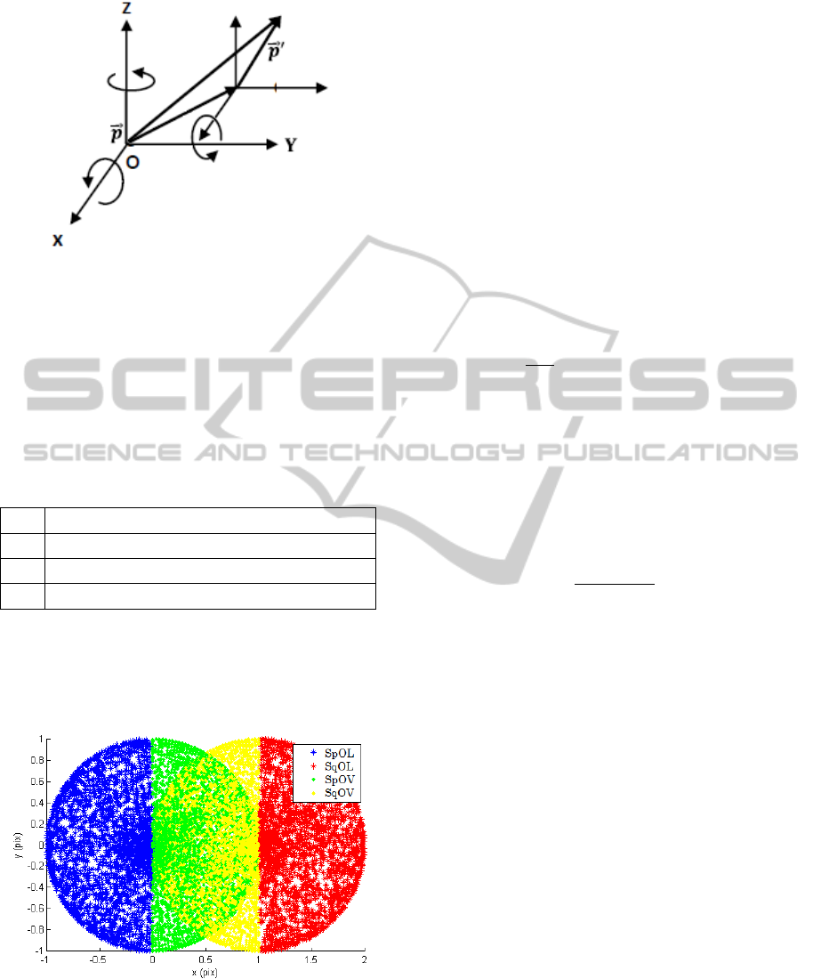
Figure 1: Sign convention for a transformation of a point
with positive parameters.
of the registration in function of the quantity of
points paired, the total error of the pairing and the
overlapping region obtained.
The sub-spaces necessary to evaluate the fitness
function are described in Table 1 and shown in
Figure 2.
Table 1: Sub-spaces defined to evaluate the fitness
function.
Overlapping points in floating cloud.
Points of floating cloud within the outlying area.
Overlapping points in fixed cloud.
Points of fixed cloud within the outlying area.
It can be seen from Figure 2 that overlapping
areas do not frame exactly the overlaid regions of
the two circles. This error is allowed due to a
threshold distance necessary for the correct
performance of the algorithm.
Figure 2: Sub-spaces for outlier and overlapping points for
two unit circles.
The fitness for each chromosome is defined
as
(
)
=
|
−
Υ
−
|
(5)
where
represents the minimum average distance
between outlier points,
is the minimum average
distance between the overlapping regions, Υ is an
adjustment factor due to the ratio of successful
pairing and is an error term due to the sampling
process.
To compute parameter
it is necessary to
calculate the individual Euclidean distances from
any point in the
space to every point in the
set and save the minimum distance. A pairing or
matching takes place if the minimum distance
obtained is less than a threshold ℎ previously
established. Once a closest neighbor has been found,
points from both sets are deleted. Repeating this
process for every point in the set
yields
=
1
,
(6)
where
(
,
)
represents a vector containing the
Euclidean distances between point and set and
is the number of elements in
. The same
procedure is followed to compute
.
Each time a point matching occurs, a counter
(initially set to zero) will be increased by two.
Parameter Υwill then be given by
Υ
=
λ
+
(7)
This last term represents exactly the ratio of
points successfully matched in the overlapping
surfaces and is used to reduce the weight of the
in order to reward a good ratio even if distances
between the overlapping points are big.
3.3 Genetic Operators
Another important factor to ensure the convergence
of the GA is the election of the right operators to act
upon the population. Such operators are selection,
crossover and mutation. This is a particular difficult
choice, given the fact that a certain combination
might work perfectly in a problem and completely
fail in another, depending on their nature.
In this section, the parameters chosen are briefly
explained. Many other variations of these operators
can be found on (Chambers, 1995) and (Goldberg,
1977).
3.3.1 Selection
In the case of a registration problem, it is
recommended to choose a selection method that
THREE-DIMENSIONAL POINT-CLOUD REGISTRATION USING A GENETIC ALGORITHM AND THE
ITERATIVE CLOSEST POINT ALGORITHM
549

applies little pressure on the population since even
the less fitted individuals could provide important
data for the optimization. A complete analysis on the
selection operator can be found on (Baker, 1989).
It was chosen to use a selection by lineal ranking
because it allows offspring from most part of the
population depending on a parameter. The first
step is to order the individuals according to their
fitness’s and calculate a new fitness based on the
function
′
()
=−
()
for =0…
−1
(8)
This assigns a value of to the less fitted
individual and a value close to
for the best
one.
Once
has been computed, a roulette selection
is used to decide on the parents that will give rise to
the new offspring. Additionally, the selection can be
set to be elitist, that is, to preserve some of the best
fitted individuals in order to maintain the minimum
fitness stable.
3.3.2 Crossover
Crossover refers to the operation of exchanging
information with a certain probability between two
individuals, namely parents. Many crossover
methods are described in (Chambers, 1995). Given
the short length of the chromosome used in this
work, a single point crossover has been chosen, with
the crossing point chosen randomly. However, to
introduce new information, the crossover model
introduced by (Radcliff, 1991) has been applied as
well. This model considers adding a random variable
to each gene based on the data from their parents,
this is
=
+(1−)
(9a)
=
(1−)+
(9b)
where
and
represent the values for the new
genes, is the random variable within the range
[0,1] and
and
are the current values of the
genes from the first and second parents, respectively.
3.3.3 Mutation
Like crossover, mutation is a critical operator for the
correct execution of a GA. Mutation introduces new
information and can be determining to converge to
the global optimum. Under mutation, each gene has
a probability of changing its value.
In binary coding, mutation consists on changing
1’s to 0’s and vice versa. A continuous coding
requires adding or subtracting a random value from
the current value of the gene within a given range.
This work considers a dynamic range of mutation,
based on the maximum fitness value and the overall,
the new value for the gene
will be given by
=·2−
−1−
(10)
where is again a random variable whose range
depends on the nature of the gene (rotation or
translation), is the current generation,
is the
average fitness of the previous generation, and
is the maximum fitness of the previous generation.
The constant 2is selected so that the new value is
constraint within the interval [0, 2], being the first
expected in the later generations.
An analysis on the advantages of choosing a
dynamic mutation model is better explained in
(Chow, 2004).
4 EXPERIMENTAL RESULTS
The proposed method was tested on three different
sets: a) a simulated surface generated and sectioned
in MATLAB, b) a model acquired by projecting
fringes over a surface and sectioned in MATLAB
and c) a model acquired by the same means as b)
and fully reconstructed to compare with the
reconstruction obtained with a commercial 3D
scanner.
4.1 Computer Simulated Surface
First, a graphic was generated using the function
PEAKS with a size of 200×200 which then was
sectioned in a floating and a fixing cloud, each one
formed by 125 pixels. Both surfaces were
standardized to a range [-0.5, 0.5] in their x and y
axis and to [-1, 1] in their z axis.
After standardizing, the floating cloud was
transformed with random parameters as mentioned
in Eq. (4a). The rotations were within the range
[-120, 120] and the displacements in [-1, 1].
The experiment was repeated ten times, of which
three are shown in Table 2. The error is measured as
the total average distance between the overlapping
points. A result of one of the experiments is shown
in Figure 3.
4.2 Real Surface Synthetically
Sectioned
A frontal view of a real surface was digitalized using
FEC 2011 - Special Session on Future of Evolutionary Computation
550
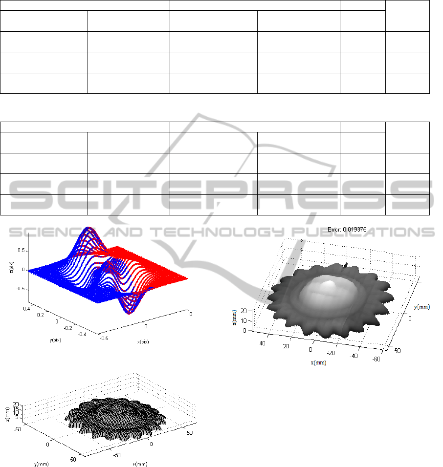
Table 2: Results obtained from registering a computer simulated surface under random transformations.
Original Obtained Error
Time(s)
(,,) (
,
,
) (,,) (
,
,
)
initial
(final)
(33.50, 90.81, -44.41) (0.09, -0.71, 0.70) (35.48, 88.31, 45.49) (0.12, -0.73, 0.68)
0.4927
(0.00373)
237.57
(59.53, -50.61, -
117.94)
(-0.52, -0.75, -0.63)
(58.72, -49.87,
116.29)
(-0.49, -0.76, -0.63)
0.5397
(0.00197)
217.64
(-5.83, 3.63, 82.47) (0.46, 0.25, 0.84) (-6.19, -3.28, -83.14) (0.428, 0.23, 0.82)
0.4756
(0.00104)
219.83
Table 3: Results obtained from registering a real surface under random transformations.
Original Obtained Error
Time(s)
(,,) (
,
,
) (,,) (
,
,
)
initial
(final)
(39.11, 2.89, 111.02) (-69.74, -29.34,
15.97)
(37.38, 1.68, 107.73) (-66.28, -30.73,
17.06)
35.2532
(0.04661)
385.73
(37.76, 48.69, 99.78) (-56.34, -31.01,
6.56)
(38.76, 48.91, 96.38) (-58.08, -31.92,
5.68)
39.6762
(0.03982)
374.29
(101.06, 49.83,
35.06)
(-65.01, 48.87,
60.75)
(99.34, 47.92, 34.73) (-63.83, 49.23,
62.38)
47.2784
(0.04251)
382.95
Figure 3: Result obtained form first experiment.
Figure 4: Range image obtained from a real surface.
a fringe projection system. The range image
obtained is shown in Figure 4. The same procedure
of sectioning and transforming was followed to
produce the differently modified clouds with a range
of displacements of [-70, 70].
The experiment was again repeated ten times and
three of the results obtained are detailed in Table 3
and one of them shown in Figure 5.
Figure 5: One of the result after applying the proposed
method.
The error is measured once again as the total
average distance between the overlapping surfaces.
4.3 Real Surface Reconstructed
For the last experiment, an object was digitalized
and fully reconstructed from four different
acquisitions. The reconstructed object was then
compared against the result of the same object
obtained with a commercial 3D scanner, being these
the floating and fixed clouds, respectively. The
acquisition was done using structured light
projection and reconstructed with the proposed
method. The final result of this experiment is shown
in Figure 6.
Both clouds were paired with an average error of
0.000116 mm/point. The reconstruction process took
THREE-DIMENSIONAL POINT-CLOUD REGISTRATION USING A GENETIC ALGORITHM AND THE
ITERATIVE CLOSEST POINT ALGORITHM
551
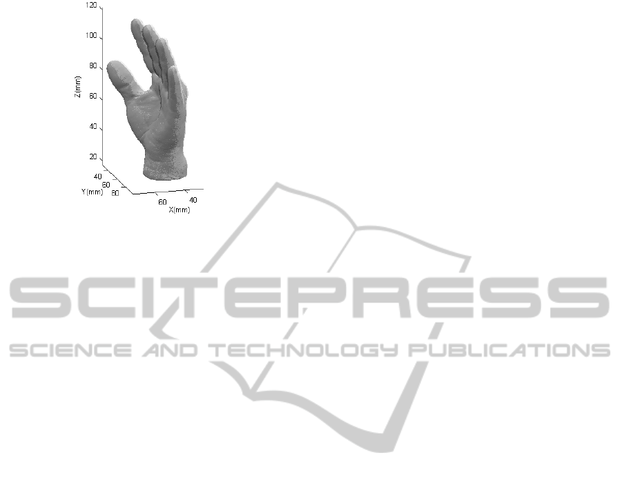
Figure 6: Surface reconstructed (light) and surface
acquired with a commercial scanner (dark).
738.47 seconds and the final pairing ended in 283.38
seconds.
5 CONCLUSIONS
The proposed method works well for dense clouds
(of about 300,000 points) and has proven its
efficiency in reconstructing tasks particularly for big
objects where many acquisition steps are needed.
With little refinement, it can also be used to compare
CAD modeled pieces with pieces machined in the
real world to give a better quality control where high
precision is needed.
REFERENCES
Arun, K. S., Huang, T. S., Blostein, S. D., 1987. In IEEE
Transactions on Pattern Analysis and Machine
Intelligence. IEEE.
Baker, J. E., 1989. Ph. D. Thesis. Vanderbilt University
Neville.
Besl, P. J., McKay, N. D., 1992. In IEEE Trans. Pattern
Anal. Machine Intel. 14.
Brunnstrom, K., Stoddart, A. J., 1996. In Proceedings of
the 13
th
International Conference on Pattern
Recognition. IEEE.
Chambers, L. D., 1995. The Practical Handbook of
Genetic Algorithms: New Frontiers Volume II. CRC
Press.
Chow, C. K., Tsui, H.T., Lee, T., 2004. In Journal of the
Pattern Recognition Society. Elsevier Science.
Friedman, J. H., Bentley, J. L., Finkel, R. A., 1977. In
ACM Trans. On Mathematical Software. ACM.
Goldberg, D. E., 1989. Genetic Algorithms in Search,
Optimization & Machine Learning.Addison-Weasley.
Masuda, T., Sakaue, K., Yokoka, N., 1996. In Proceedings
of the 13th International Conference on Pattern
Recognition. IEEE.
Pottmann, H., Leopoldseder, S., Hofer, M., 2004. In
Computer Vision and Image Understanding 95.
Elsevier Science.
Robertson, C., Fisher, R. B., 2001. In Journal of Computer
Vision and Image Understanding 87. Elsevier Science.
FEC 2011 - Special Session on Future of Evolutionary Computation
552
