SIMULATED ANNEALING METHOD WITH DIFFERENT

NEIGHBORHOODS FOR SOLVING THE

CELL FORMATION PROBLEM

Luong Thuan Thanh

, Jacques A. Ferland

1,2

, Nguyen Dinh Thuc

and Van Hien Nguyen

1,4

(ICST HCMC), Institute for Computational Science and Technology, Ho Chi Minh City, Vietnam

Department of Computer Science and Operations Research, University of Montreal, Montreal, Canada

Faculty of Information Technology, University of Science, Vietnam National University, Ho Chi Minh City, Vietnam

Department of Mathematics, University of Namur (FUNDP), Namur, Belgium

Keywords: Cell formation problem, Metaheuristic, Simulated annealing, Diversification, Intensification, Neighbor-

hood.

Abstract: In this paper we solve the cell formation problem with different variants of the simulated annealing method

obtained by using different neighborhoods of the current solution. The solution generated at each iteration

is obtained by using a diversification of the current solution combined with an intensification to improve

this solution. Different diversification and intensification strategies are combined to generate different

neighborhoods. The most efficient variant allows improving the best-known solution of one of the 35

benchmark problems commonly used by authors to compare their methods, and reaching the best-known

solution of 30 others.

1 INTRODUCTION

The Group Technology is an approach often used in

manufacturing and engineering management taking

advantage of similarities in production design and

processes. In this context, the Cellular

Manufacturing refers to maximize the overall

efficiency of a production system by grouping

together machines providing service to similar parts

into a subsystem (denoted cell). The corresponding

problem is formulated as a (Machine-Part) Cell

Formation Problem. As a consequence, the

interactions of the machines and the parts within a

cell are maximized, and those between machines and

parts of other cells are reduced as much as possible.

The cell formation problem is a NP hard

optimization problem (Dimopoulos and Zalzala,

2000). For this reason, several heuristic methods

have been developed over the last forty years to

generate good solutions in reasonable computational

time. To learn more about the different methods, we

refer the reader to the survey papers proposed in

(Goncalves and Resende, 2004), and in

(Papaioannou and Wilson, 2010) where the authors

survey the different techniques classified as follows:

• Cluster analysis: techniques for recognizing

structure in a data set

• Graph partitioning approaches where a

graph or a network representation is used to

formulate the cell formation problem

• Mathematical programming methods: the

cell formation problem is formulated like a

non linear or linear integer programming

problem

• Heuristic, metaheuristic and hybrid

metaheuristic: The most popular methods

are: simulated annealing, tabu search,

genetic algorithms, colony optimization,

particle swarm optimization, neural

networks and fuzzy theory.

In (Ghosh et al., 2010), the authors introduce a

survey of various genetic algorithms used to solve

the cell formation problem. The success of genetic

algorithms in solving this problem induced

researchers to consider different variants and

hybrids in order to generate very robust techniques.

In this paper, we introduce solution methods

hybridizing different approaches. These methods are

variants of the simulated annealing (Kirkpatrick et

al., 1983, Cerny,1994) using different neighbor-

525

Thanh L., A. Ferland J., Thuc N. and Nguyen V..

SIMULATED ANNEALING METHOD WITH DIFFERENT NEIGHBORHOODS FOR SOLVING THE CELL FORMATION PROBLEM.

DOI: 10.5220/0003723705250533

In Proceedings of the International Conference on Evolutionary Computation Theory and Applications (FEC-2011), pages 525-533

ISBN: 978-989-8425-83-6

 2011 SCITEPRESS (Science and Technology Publications, Lda.)

hoods of the current solution. The solution generated

at each iteration is obtained by using a

diversification of the current solution combined with

an intensification to improve this solution. Different

diversification and intensification strategies are

combined to generate different neighborhoods.

Numerical results are obtained to compare

numerically the efficiency of the variants with

respect to the best-known solutions of 35 benchmark

problems commonly used by authors to evaluate

their methods.

The cell formation problem is summarized in

Section 2. Section 3 is devoted to the simulated

annealing procedure. We introduce the different

diversification and intensification strategies to

develop the different neighborhoods. The numerical

results are summarized in Section 4. The most

efficient variant allows to improve the best-known

solution of one problem and to reach it for 30 other

problems.

2 PROBLEM FORMULATION

To formulate the cell formation problem, consider

the following two sets

set of machines: 1, ,

set of parts: 1, , .

mim

Jnjn

…

The production incidence matrix

[

]

a= indicates

the interactions between the machines and the parts:

1 if machine process part

0 otherwise.

a =

⎧

⎨

⎩

Furthermore, a part j may be processed by several

machines. A production cell k

()

1, ,kK= …

includes a subset (group) of machines

CI⊂ and a

subset (family) of parts

J⊂ . The problem is to

determine a solution including K production cells

()( )( ){

}

,= ,,, ,

CF C F C F… as autonomous as

possible. Note that the K production cells induce

partitions of the machines set and of the parts set:

{}

12 12

and

and for all pairs of and 1, ,

and .

kk kk

CCI FFJ

kk K

CC FF

φφ

∈

≠

∪…∪ ∪…∪

…

∩∩

To illustrate the production cells concept, consider a

machine-part incidence matrix in Table 1. Table 2

indicates a partition into 3 different cells illustrated

in the gray zones. The solution includes the 3

machine groups {(1,4,6), (3,5), (2)} and the 3 part

families {(2,4,6,8), (1,7), (3,5)}.

Table 1: Incidence matrix.

Parts 1 2 3 4 5 6 7 8

Machines

1 0 1 0 1 1 1 0 1

2 1 0 1 0 1 0 0 0

3 1 0 1 0 0 0 1 0

4 0 1 0 1 0 1 0 1

5 1 0 0 0 0 0 1 1

6 1 1 0 0 0 1 1 1

Table 2: Matrix solution.

Parts 2 4 6 8 1 7 3 5

Machines

1 1 1 1 1 0 0 0 1

4 1 1 1 1 0 0 0 0

6 1 0 1 1 1 1 0 0

3 0 0 0 0 1 1 1 0

5 0 0 0 1 1 1 0 0

2 0 0 0 0 1 0 1 1

The exceptional elements (1,5), (6,1), (6,7), (3,3),

(5,8) and (2,1) correspond to entries having a value

1 that lay outside of the gray diagonal blocks.

Sarker and Khan, (2001) carry out a comparative

study of different autonomy measures for the

solution of a cell formation problem. In this paper

we consider the grouping efficacy Eff (Kumar and

Chandrasekharan, 1990) that is mostly used:

Out In

nIn

aa a

Eff

aa aa

−

where

∑

denotes the total number of

entries equal to 1 in the matrix A,

Out

a denotes the

number of exceptional elements, and

and

nIn

aaare

the numbers of one and of zero entries in the gray

diagonal blocks, respectively. The objective

function of the problem is maximizing

Eff .

In our numerical experimentation we fix the

number K of cells for each problem to its value in

the best-known solution reported in the literature.

3 SIMULATED ANNEALING

The local search procedure used to solve the cell

FEC 2011 - Special Session on Future of Evolutionary Computation

526

formation problem is a straightforward

implementation of the simulated annealing method

presented in (Ferland and Costa, 2001), but the

different neighborhoods are specific for the

problem.

Procedure Simulated Annealing (N)

Initialization:

Let

()

,CF an initial solution;

TP the initial

temperature

Let

iter : 0; : ; : 0TP TP fcount== =

Let

()

()()

** 00

, : , : , ; stop : falseCF C F C F== =

While not stop

:0; :0changes trials==

While trials SF< and changes coff<

Generate a solution

()()

,,CF NCF

′′

∈

()

(

)

:, ,Eff C F Eff C F

′′

Δ= −

0Δ>

then

()( )

,: ,CF C F

′′

and changes := changes + 1

else generate a random number

()

0,1r ∈

/ TP

< then

()( )

,: ,CF C F

′′

and changes := changes + 1

()

(

)

,,Eff C F Eff C F

′′

> then

()

,: ,CF CF

′

and fcount := 0

trials := trials + 1

:TP TP

Iter := iter + 1

If changes/trials < mpc then

fcount := fcount + 1

If iter ≥ itermax or fcount = flimit then

stop := true

()

,CF is the best solution generated



In this variant of the simulated annealing, we

complete several iterations with the same

temperature

TP. This temperature is modified when

the number of trial solutions (

trials) or when the

number of times that the current solution is changed

(

changes) reaches threshold values Sf or coff,

respectively. The parameter

is used to modify the

temperature. Two stopping criteria are used. The

first is fixed in terms of the number of different

temperature values used (itermax). To apply the

second criterion, we keep track of the number of

consecutive temperature values (

fcount) where the

number of

changes over the number of trials is

smaller than a threshold value mpc. When

fcount

reaches the value

flimit, the procedure stops.

To complete the presentation of the procedure,

we indicate how the initial solution

()

,CF is

generated and the different neighborhoods

N that we

are using.

3.1 Initial Solution

To generate the initial solution, we use a procedure

quite similar to the one proposed in (Rojas

et al.,

2004) that is introduced in (Elbenani

et al., 2010).

First we determine K machine groups

CC… .

Then the

K part families

F… are specified on

the basis of the

K machines groups known.

Denote :

and

iijjij

aaa a

∑

the number of parts processed by machine

i and the

number of machines processing

j, respectively. To

initiate the machine groups formation, select the

machines having the largest values

, and assign

them to the different groups

,1, .

Ck K= …

Then

each of the other machines left is assigned to the

group

C including machines processing mostly the

same parts.

On the basis of the

K machine groups

CC… ,

determine the

K part families

F… . For each

part

j, denote

(

)

the number of machines

in group that are processing part

jij

ak a

∈

•=

∑



(

)

(

)

the number of machines

in group that are not processing part

In In

jkj

ak C ak

•=−



SIMULATED ANNEALING METHOD WITH DIFFERENT NEIGHBORHOODS FOR SOLVING THE CELL

FORMATION PROBLEM

527

()

an approximation of the impact on

the grouping efficiency of assigning

part to family .

aak

Eff

•



()

Then each part is assigned to the family



()

1, ,

where ArgMax

aak

⎧⎫

⎨⎬

⎩⎭

…



in order to

generate a good initial solution

()

,CF having the

grouping efficiency

()

akj

Eff C F

aakj

∑



3.2 Neighborhoods

Different neighborhoods are used to obtain different

variants of the simulated annealing method. Each

neighborhood is obtained by using a diversification

strategy to destroy and recover a new solution, and

an intensification strategy to improve the new

solution. This solution generated is denoted

()()

,,CF NCF

′′

∈ .

3.2.1 Diversification of the Solution

(

)

,CF

The procedure is applied on the current solution

()

,CF in order to modify (destroy) the assignment

of some elements (machines and/or parts) to be

reassigned to other cells selected randomly in order

to recover a new solution

()

,CF

′′ ′′

. We consider

two different ways to destroy the current solution

()

,CF :

•

D1: Modify the assignment of %n

⎡⎤

⎢⎥

parts and

⎡⎤

⎢⎥

machines (% being a parameter

of the method).

•

D2: Select randomly between two strategies:

modify either

⎡⎤

⎢⎥

parts or modify

⎡⎤

⎢⎥

machines.

3.2.2 Intensification of the Solution

()

,CF

′

′′′

To intensify the search around the solution

()

,CF

′′ ′′

, we modify successively the machine

groups on the basis of the part families and the part

families on the basis of the machine groups until no

modification is possible. The solution

(

)

(

)

,,CF NCF

′′

∈ is the best solution generated

during the process. In this paper we consider two

different ways for doing the intensification.

I1: Local Search Algorithm:

This intensification strategy is introduced in

(Elbenani

et al., 2011). The procedures to modify

the machine groups on the basis of the part families

and to modify the part families on the basis of the

machine groups are similar to the process for fixing

the part families on the basis of the machine groups

introduced in the preceding Section 3.1 (where we

generate the initial solution).

Note that whenever the machines groups (or the

part families) include an empty one, then we apply a

repair process to reassign one machine to it

inducing the smallest decrease of the grouping

efficiency.

I2: Exact Procedure:

The exact procedure relies on the Dinkelbach

approach for solving the problem of generating part

families on the basis of the machine groups. This

procedure can be adapted

mutatis mutandis for the

problem of generating machine groups on the basis

of the part families. Since the definition of the group

efficiency

Out In

nIn

aa a

Eff

aa aa

−

is fractional, the Dinkelbach approach is appropriate

because the problem of generating the part families

on the basis of the machines reduces to solving a

sequence of problems where the objective function

has the form

()

In In

Ea aa

λλ

=− +

for a sequence of values

{

}

that are generated

during the solution process in order to obtain an

optimal value of

.Eff This procedure is even more

efficient since the problem of maximizing the value

(

)

is trivial to solve once the machine groups

are specified. To reduce the length of the paper, we

are not presenting the details of the procedure that

can be found in (Khoa

et al., 2011).

3.2.3 Four Different Neighborhoods

In this paper we compare numerically four different

variants specified using the following

FEC 2011 - Special Session on Future of Evolutionary Computation

528

neighborhoods:

N : generated with the diversification D1 and the

intensification

N : generated with the diversification D1 and the

intensification

N : generated with the diversification D2 and the

intensification

N : generated with the diversification D2 and the

intensification

I2.

4 NUMERICAL RESULTS

To complete the numerical experimentation, we

consider 35 benchmark problems that are commonly

used by authors to evaluate the efficiency of their

methods. The first 5 columns of Table 3 indicate the

problem number, the reference where it is specified

(Problem source), its size (values of

m, n, and K),

and the value of its best-known solution (Best-

known solution). Moreover the values of the best-

known solutions are identified by refereeing to the

following references (Goncalves and Resende, 2004,

James

et al., 2007, Luo and Tang, 2009, Mahdavi et

al.

, 2007, Tunnukij and Hicks, 2009, Elbenani et al.,

2010, and Ying

et al., 2011).

The purpose of this analysis is twofold. First we

compare the average group efficiency over 10 runs

obtained with the simulated annealing method using

the four neighborhoods with the best-known

solutions for the 35 benchmark problems. As a

consequence we should identify the best

diversification (

D1 or D2) and the best

intensification (

I1 or I2) strategies. In the second

part, we compare the impact of the percentage % of

modified elements in the diversification strategies.

Three different values are considered: 20%, 30%,

and 50%.

The numerical tests are completed on a PC

equipped with an INTEL Core 2 Duo processor

running at 2.2 GHZ, and having a 2 GB of central

memory on a Linux system. The parameters to

implement the simulated annealing method are as

follows:

100 mpc 0.5

2 itermax 10

20.2

TP K

Sf K K

coff K

flimit =

The last four columns of Table 3 include the average

grouping efficiency over 10 runs of the simulated

annealing method using the four different

neighborhoods

,1,,4.

Ni= … For each problem,

the best solution is marked in bold. To reduce the

length of the paper, we report only the table where

the percentage is fixed at 30%, but the tables for the

other two values of % are quite similar. The

numerical results in Table 3 indicate that the variants

using neighborhoods

and NNallows to generate

better results than using

and NN. The variants

and NN

generate a solution better that the best-

known solution of P33, and the number of problems

where the best-known solution is reached is equal to

30 and 29 for

N and

N , respectively.

Furthermore, the overall averages (last row of the

Table 3) for the variants with

N and

N are at

0.030 % and 0.045%, respectively, from the overall

average of the best-known solutions. Hence these

variants seem very efficient to solve the cell

formation problem.

This analysis above allows to conclude that the

intensification strategy

I2 seems more efficient than

I1. Furthermore, since the variant

N is slightly more

efficient than

N , it follows that the diversification

D1 seems to be slightly more efficient than D2 when

combined

with the intensification I2.

Now consider the results summarized in Table 4

to analyze the efficiency of the variant using

N when using the different percentages %. For

each problem, the best-solution is marked in bold,

and the smallest solution time is marked in italic

bold.On the one hand, as far as the average grouping

efficiency is concerned, the percentage 30% allows

to generate slightly better results: the three

percentages allow generating solutions having the

same overall average (last row of the Table 4) of

65.95, but the number of problems where the best-

known solution is reached or exceeded is 29, 31, and

30 for the values 20%, 30%, and 50%, respectively.

On the other hand, using the percentage 20% allows

an average solution time (12.03 sec.) smaller that of

the other percentages (14.73 sec. for 30% and

19.15sec. for 50%). Thus if the user put more

emphasis on the quality of the solution, then the

percentage 30% is more appropriate, but if the

solution time must be reduced, then the percentage

of 20% is more convenient.

SIMULATED ANNEALING METHOD WITH DIFFERENT NEIGHBORHOODS FOR SOLVING THE CELL

FORMATION PROBLEM

529

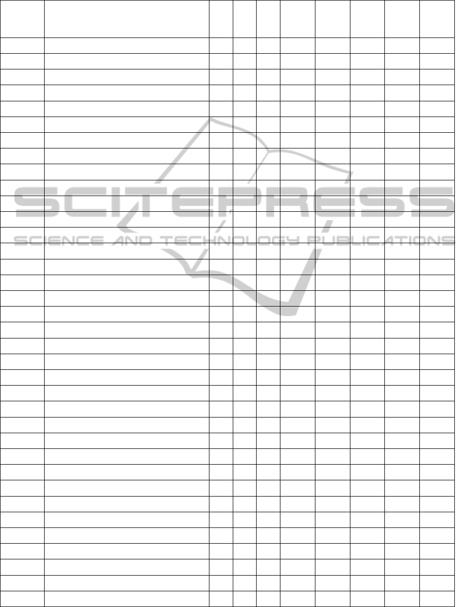
Table 3: Compare grouping efficiency of the four neighborhoods when %=30%.

Problem

number

Problem source m n K

Best-

know

P1 King and Nakornchai (1882) 5 7 2

82.35 82.35 82.35 82.35 82.35

P2 Waghodekar and Sahu (1984) 5 7 2

69.57

69.25

69.57

69.41

69.57

P3 Seifoddini (1989) 5 18 2

79.59 79.59 79.59 79.59 79.59

P4 Kusiak and Cho (1992) 6 8 2

76.92 76.92 76.92 76.92 76.92

P5 Kusiak and Chow (1987) 7 11 5

60.87 60.87 60.87 60.87 60.87

P6 Boctor (1991) 7 11 4

70.83 70.83 70.83 70.83 70.83

P7 Seifoddini and Wolfe (1986) 8 12 4

69.44 69.44 69.44

68.84

69.44

P8 Chandrasekharan and Rajagopalon (1986a) 8 20 3

85.25 85.25 85.25 85.25 85.25

P9 Chandrasekharan and Rajagopalon (1986b) 8 20 2

58.72

58.62 58.56 58.4 58.5

P10 Mosier and Taube (1985a) 10 10 5

75 75 75 75 75

P11 Chan and Milner (1982) 10 15 3

92 92 92 92 92

P12 Askin and Subramanian (1987) 14 24 7

72.06

71.64

72.06

71.54

72.06

P13 Stanfel (1985) 14 24 7

71.83 71.83 71.83 71.83 71.83

P14 McCormick (1972) 16 24 8

53.26

52.96

53.26

52.83

53.26

P15 Srinivasan et al. (1990) 16 30 6

69.53

67.83

69.53

68.02 69.11

P16 King (1980) 16 43 8

57.53

57.41

57.53

57.38

57.53

P17 Carrie (1973) 18 24 9

57.73 57.73 57.73 57.73 57.73

P18 Mosier and Taube (1985b) 20 20 5

43.45

43.01 43.12 42.83 43.06

P19 Kumar et al. (1986) 20 23 7

50.81 50.81 50.81

50.68

50.81

P20 Carrie (1973) 20 35 5

77.91

76.33

77.91

76.33

77.91

P21 Boe and Cheng (1991) 20 35 5

57.98

56.93

57.98

56.86

57.98

P22 Chandrasekharan and Rajagopalon (1989) 24 40 7

100 100 100 100 100

P23 Chandrasekharan and Rajagopalon (1989) 24 40 7

85.11 85.11 85.11 85.11 85.11

P24 Chandrasekharan and Rajagopalon (1989) 24 40 7

73.51 73.51 73.51 73.51 73.51

P25 Chandrasekharan and Rajagopalon (1989) 24 40 11

53.29 53.29 53.29 53.29 53.29

P26 Chandrasekharan and Rajagopalon (1989) 24 40 12

48.95 48.95 48.95

48.85

48.95

P27 Chandrasekharan and Rajagopalon (1989) 24 40 12

47.05

46.57 46.58 46.52 46.55

P28 McCormick (1972) 27 27 5

54.82 54.82 54.82

54.78

54.82

P29 Carrie (1973) 28 46 10

47.08

46.39

47.08

46.23

47.08

P30 Kumar and Vannelli (1987) 30 41 14

63.31

62.99

63.31

62.9

63.31

P31 Stanfel (1985) 30 50 13

60.12 60.12 60.12

60.09

60.12

P32 Stanfel (1985) 30 50 14

50.83

50.8

50.83

50.74

50.83

P33 King and Nakornchai (1982) 36 90 17 47.75 47.65

47.98

47.61

47.98

P34 McCormick (1972) 37 53 3

60.64

58.31 60.63 58.26 60.63

P35 Chandrasekharan and Rajagopalon (1987) 40

84.03 84.03 84.03 84.03 84.03

Average 65.97 65.68 65.95 65.64 65.94

FEC 2011 - Special Session on Future of Evolutionary Computation

530

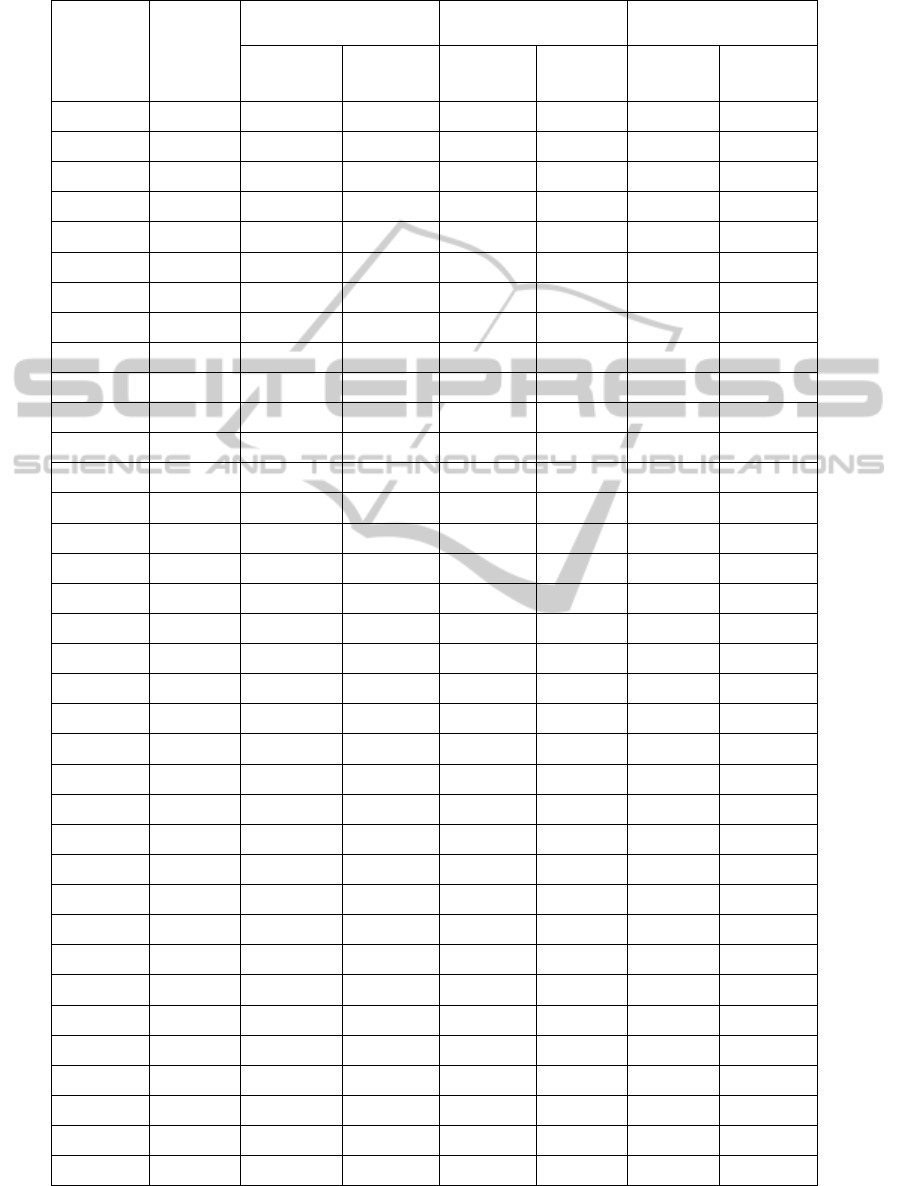
Table 4: Compare grouping efficiency of

N when %=20% , 30% and 50%.

Problem

number

Best

Known

Solution

(20%)N

(30%)N

(50%)N

Average

Eff

Solution

time

Average

Eff

Solution

time

Average

Eff

Solution

time

82.35 82.35

0.018

82.35

0.027

82.35

0.037

69.57 69.57

0.02

69.57

0.028

69.57

0.03

79.59 79.59

0.037

79.59

0.048

79.59

0.053

76.92 76.92

0.026

76.92

0.028

76.92

0.037

60.87 60.87

0.374

60.87

0.426

60.87

0.465

70.83 70.83

0.227

70.83

0.245

70.83

0.313

69.44 69.44

0.251

69.44

0.28

69.44

0.329

85.25 85.25

0.146

85.25

0.166

85.25

0.203

58.72

58.53

0.045

58.56 0.051 58.68 0.056

P10

75 75

0.421

0.493

0.628

P11

92 92

0.14

0.154

0.193

P12

72.06 72.06

2.252

72.06

2.735

72.06

3.234

P13

71.83 71.83

2.206

71.83

2.755

71.83

3.271

P14

53.26 53.26

4.83

53.26

5.22

53.26

6.107

P15

69.53 69.53

1.621

69.53

1.904

69.53

2.432

P16

57.53 57.53

6.932

57.53

7.759

57.53

8.837

P17

57.73 57.73

6.288

57.73

7.34

57.73

8.461

P18

43.45

43.04

1.398

43.12 1.702 43.06 2.157

P19

50.81 50.81

3.336

50.81

3.8

50.81

4.699

P20

77.91 77.91

1.254

77.91

1.484

77.91

1.895

P21

57.98 57.98

1.483

57.98

1.764

57.98

2.233

P22

100 100

4.284

100

4.362

100

5.196

P23

85.11 85.11

4.423

85.11

4.865

85.11

7.3

P24

73.51 73.51

4.637

73.51

5.502

73.51

8.439

P25

53.29 53.29

15.459

53.29

19.5

53.29

25.688

P26

48.95 48.95

21.828

48.95

29.264 48.89 39.328

P27

47.05

46.58

21.194

46.58 27.573 46.47 44.499

P28

54.82 54.82

1.306

54.82

1.631

54.82

1.98

P29

47.08

47.07

21.323

47.08

22.886

47.08

30.358

P30

63.31

63.29

47.698

63.31

58.074

63.31

65.067

P31

60.12 60.12

32.113

60.12

39.162

60.12

51.728

P32

50.83 50.83

47.931

50.83

55.442

50.83

78.725

P33 47.75

47.96

135.463

47.98

177.951

47.97

220.549

P34

60.64

60.63

1.008

60.63 1.021 60.63 1.07

P35

84.03 84.03

29.171

84.03

30.058

84.03

44.561

Average 65.97 65.95 12.03 65.95 14.73 65.95 19.15

SIMULATED ANNEALING METHOD WITH DIFFERENT NEIGHBORHOODS FOR SOLVING THE CELL

FORMATION PROBLEM

531

5 CONCLUSIONS

The cell formation problem is solved with the

simulated annealing method where the solution in

the neighborhood of the current solution is obtained

by using a diversification strategy to destroy and

recover a new solution, and an intensification

strategy to improve the new solution.

We consider

two different diversification strategies to destroy the

current solution

()

,CF :

• D1: Modify the assignment of %n

⎡⎤

⎢⎥

parts and

⎡⎤

⎢⎥

machines

• D2: Select randomly between two strategies:

modify either

⎡⎤

⎢⎥

parts or modify

⎡⎤

⎢⎥

machines

where the parameter % takes the values 20%, 30%,

or 50%. Two different intensification strategies are

specified as follows:

• I1: Local search algorithm introduced in

(Elbenani et al., 2011)

• I2: Exact procedure based on the Dinkelbach

method.

Different variants combining a diversification and

an intensification are compared numerically with the

best-known solution of 35 benchmarked problems

commonly used by authors to compare the

efficiency of their method. The most efficient

variant using the diversification

D2 with 30%

destroying rate and the intensification

I2 allows to

improve the best-known solution of one problem

and to reach it for 30 other problems.

We are now implementing adaptive methods

where the selection of the diversification and the

intensification strategies is modified during the

solution procedure. The selection should be made

randomly according to probabilities assigned to the

strategies that are proportional to their efficiency up

to this point.

REFERENCES

Askin, R. G. and Subramanian, S. P., 1987. A cost-based

heuristic for group technology configuration.

International Journal of Production Research, 25,

101–113.

Boctor, F. F., 1991. A linear formulation of the machine-

part cell formation problem.

International Journal of

Production Research

, 29, 343–356.

Boe, W. J. and Cheng, C. H., 1991. A close neighbour

algorithm for designing cellular manufacturing

systems.

International Journal of Production

Research

, 29, 2097–2116.

Carrie, A. S., 1973. Numerical taxonomy applied to group

technology and plant layout.

International Journal of

Production Research

, 11, 399–416.

Cerny, V., 1985. Thermodynamical approach to the

traveling salesman problem: an efficient simulation

algorithm.

Journal of Optimization Theory and

Application

, 45, 41 – 51.

Chan, H. M. and Milner, D. A., 1982. Direct clustering

algorithm for group formation in cellular manufacture.

Journal of Manufacturing Systems, 1, 65-75.

Chandrasekharan, M. P. and Rajagopalan, R., 1987.

ZODIAC: an algorithm for concurrent formation of

part-families and machine-cells.

International Journal

of Production Research

, 25, 835–850.

Chandrasekharan, M. P. and Rajagopalan, R., 1989.

GROUPABILITY: an analysis of the properties of

binary data matrices for group technology.

International Journal of Production Research, 27,

1035–1052.

Chandrasekharan, M. P. and Rajagopalan, R., 1986a.

MODROC: an extension of rank order clustering for

group technology.

International Journal of

Production Research

, 24, 1221–1233.

Chandrasekharan, M. P. and Rajagopalan, R., 1986b. An

ideal seed non-hierarchical clustering algorithm for

cellular manufacturing.

International Journal of

Production Research

, 24, 451–464.

Dimopoulos, C. and Zalzala, A. M. S., 2000. Recent

developments in evolutionary computations for

manufacturing optimization: problems, solutions, and

comparisons.

IEEE Transactions on Evolutionary

Computations

, 4, 93–113.

Elbenani, B., Ferland, J. A., Bellemare J., 2011. Genetic

algorithm and large neighbourhood search to solve the

cell formation problem.

Expert Systems with

Applications

(to appear).

Ferland, J. A. and Costa D., 2001. Heuristic search

methods for combinatorial programming problems.

Publication # 1193, Department of computer science

and operation research

, University of Montreal,

Canada.

Ghosh, T., Dan, P. K., Sengupta, S., Chattopadhyay, M.,

2010. Genetic rule based techniques in cellular

manufacturing (1992-2010): a systematic survey.

International Journal of Engineering Science and

Technology

, 2, 198–215.

Goncalves, J. and Resende, M. G. C., 2004. An

evolutionary algorithm for manufacturing cell

formation.

Computers & Industrial Engineering, 47,

247–273.

James, T. L., Brown, E. C., Keeling, K. B., 2007. A

hybrid Grouping Genetic Algorithm for the cell

formation problem.

Computers & Operations

Research

, 34, 2059–2079.

FEC 2011 - Special Session on Future of Evolutionary Computation

532

Khoa, T., Ferland, J. A., Tien, D., 2011. A randomized

local search algorithm for the machine-part cell

formation problem. In

Advanced Intelligent

Computing Technology and Applications-ICIC2011

(to appear).

King, J. R., 1980. Machine-component grouping in

production flow analysis: an approach using a rank

order clustering algorithm.

International Journal of

Production Research

, 18, 213–232.

Kirkpatrick, S., Gelatt, C. D. Jr, Vecchi, M. P., 1983.

Optimization by simulated annealing.

Science, 220,

671 – 680.

King, J. R. and Nakornchai, V., 1982. Machine-

component group formation in group technology:

review and extension.

International Journal of

Production Research

, 20, 117–133.

Kumar, C. and Chandrasekharan, M., 1990. Grouping

efficiency: a quantitative criterion for goodness of

block diagonal forms of binary matrices in group

technology.

International Journal of Production

Research

, 28, 233–243.

Kumar, K. R. and Vannelli, A., 1987. Strategic

subcontracting for efficient disaggregated

manufacturing.

International Journal of Production

Research

, 25, 1715–1728.

Kumar, K. R., Kusiak, A., Vannelli, A., 1986. Grouping

of parts and components in flexible manufacturing

systems.

European Journal of Operational Research,

24, 387–397.

Kusiak, A. and Cho, M., 1992. Similarity coefficient

algorithm for solving the group technology problem.

International Journal of Production Research, 30,

2633–2646.

Kusiak, A. and Chow, W. S., 1987. Efficient solving of

the group technology problem,

Journal of

Manufacturing Systems

, 6, 117–124.

Luo, L., Tang, L., 2009. A hybrid approach of ordinal

optimization and iterated local search for

manufacturing cell formation.

International Journal of

Advanced Manufacturing Technology

, 40, 362– 372.

Mahdavi, I., Javadi, B., Fallah-Alipour, K., Slomp, J.,

2007. Designing a new mathematical model for

cellular manufacturing system based on cell

utilization.

Applied Mathematics and Computation,

190, 662-670.

McCormick, W. T., Schweitzer, P. J., White, T. W., 1972.

Problem decomposition and data reorganization by a

clustering technique.

Operations Research, 20, 993–

1009.

Mosier, C. T. and Taube, L., 1985a. The facets of group

technology and their impact on implementation.

OMEGA, 13, 381–391.

Mosier, C. and Taube, L., 1985b. Weighted similarity

measure heuristics for the group technology machine

clustering problem,

OMEGA, 13, 577–83.

Papaioannou, G. and Wilson, J. N., 2010. The evolution of

cell formation problem methodologies based on recent

studies (1997-2008): Review and directions for future

research,

European Journal of Operational Research,

206, 509–521.

Rojas, W., Solar, M., Chacon, M, Ferland, J. A., 2004. An

efficient genetic algorithm to solve the manufacturing

cell formation problem. In

Adaptive Computing in

Design and Manufacture VI,

I.C. Parmee (ed),

Springer-Verlag, 173–184 .

Sarker, B. and Khan, M., 2001. A comparison of existing

grouping efficiency measures and a new grouping

efficiency measure.

IIE Transactions, 33, 11–27.

Seifoddini, H., 1989. A note on the similarity coefficient

method and the problem of improper machine

assignment in group technology applications.

International Journal of Production Research, 27,

1161–1165.

Seifoddini, H. and Wolfe, P. M., 1986. Application of the

similarity coefficient method in group technology,

IIE

Transactions

, 18, 271–277.

Srinivasan, G., Narendran, T. T., Mahadevan, B., 1990.

An assignment model for the part-families problem in

group technology,

International Journal of

Production Research

, 28, 145–152.

Stanfel, L. E., 1985. Machine clustering for economic

production.

Engineering Costs and Production

Economics

, 9, 73–81.

Tunnukij, T. and Hicks, C., 2009. An Enhanced Genetic

Algorithm for solving the cell formation problem.

International Journal of Production Research, 47,

1989–2007.

Waghodekar, P. H. and Sahu, S., 1984. Machine-

component cell formation in group technology

MACE.

International Journal of Production

Research

, 22, 937–948.

Ying K. C., Lin S.W., Lu C. C. 2011. Cell formation

using a simulated annealing algorithm with variable

neighbourhood.

European Journal of Industrial

Engineering

, 5, 22–42.

SIMULATED ANNEALING METHOD WITH DIFFERENT NEIGHBORHOODS FOR SOLVING THE CELL

FORMATION PROBLEM

533