INTERVAL AVAILABILITY ANALYSIS

OF A TWO-ECHELON, MULTI-ITEM SYSTEM

Ahmad Al Hanbali and Matthieu van der Heijden

School of Management and Governance, University of Twente, Enschede, The Netherlands

Keywords: Inventory, Spare Parts, Markov Processes, Supply Chain Management, Interval Availability.

Abstract: In this paper we analyze the interval availability of a two-echelon, multi-item system. Modeling the system

as a Markov chain we analyze the interval availability of the system. We compute in closed and exact form

the expectation and, the variance of the availability during a finite time interval [0,T]. We use these

characteristics together with the probability that interval availability is equal to one to approximate the

survival function using a Beta distribution. Comparison of our approximation with simulation shows

excellent accuracy, especially for points that are practically most relevant.

1 INTRODUCTION

Nowadays, the aftersales service business represents

a considerable part of the economy and, moreover,

is continuously growing (AberdeenGroup 2005;

Deloitte 2006).

Advanced capital goods such as MRI scanners,

lithography systems, baggage handling systems, and

radar systems, are highly downtime critical. So the

customers of these advanced goods are not just

interested in acquiring these systems at an affordable

price, but far more in a good balance between the

resulting Total Cost of Ownership (TCO) and

system productivity throughout the life cycle,

including the limitation of downtime. For customers

the system use rather than the system upkeep is their

core business. Therefore, a major part of the system

upkeep is preferably outsourced to the original

manufacturer or to a service provider that can offer a

good balance between the downtime and costs. For

that reason, service contracts are made between the

service provider and customers. These contracts

specify the services provided by the supplier with

their corresponding Service Level Agreements

(SLAs), such as the time between system failure and

time of fault resolution, and the system availability.

The SLAs are measured over a predetermined

time window, e.g., a quarter or a year. For the

service providers, it is essential that the service

levels are attained, because in some cases penalties

apply if an SLA target is violated. In case of a large

scale service contract (the average performance over

many systems is measured), the average

performance should meet the target. If the number of

systems covered by a contract is relatively small, we

have inherent statistical variability and we need an

additional buffer in performance to assure that the

probability of not meeting the SLAs over the time

window is still acceptable. We encountered such a

situation at Thales Netherlands, a manufacturer of

naval sensors and naval command and control

systems. There, a service contract typically covers a

few systems only. In the literature, this issue is

usually neglected. In this paper, we are mainly

interested in the logistical delay due to the

unavailability of spare parts. Moreover, the focus

will be on SLAs that are based on the system

availability during a predetermined period of times.

In service parts logistics there is usually a

tradeoff between the cost involved in keeping the

stocks very close to the customers sites or at a

central depot, which can supports multiple

customers at the same time. Due to the risk pooling

effect, it is more desirable from the point of a service

provider to position the stocks of spare parts

centrally. However, having a strict SLA, e.g., 99%

availability, with a customer forces the service

provider to move some spare parts closer to the

customer sites. In addition, in order to reduce the

system downtime and its critical consequences it is

usually the case that the repair of failed system is

done by replacing the failed part with a new part.

The failed part is sent to the repair shop, i.e., the

342

Al Hanbali A. and van der Heijden M..

INTERVAL AVAILABILITY ANALYSIS OF A TWO-ECHELON, MULTI-ITEM SYSTEM.

DOI: 10.5220/0003701703420348

In Proceedings of the 1st International Conference on Operations Research and Enterprise Systems (ICORES-2012), pages 342-348

ISBN: 978-989-8425-97-3

 2012 SCITEPRESS (Science and Technology Publications, Lda.)

inventory is managed using the so-called base stock

policy referred to as (s-1,s)-policy. (Sherbrooke

1968) was among the first to tackle the spare part

optimization problem. He proposed the METRIC

model that is based on the maximization of system

availability subject to a constraint on the invested

budget in spare parts. METRIC model is a good

approximation in case of multi-echelon spare part

network and especially in case of high availability.

(Graves 1985) extended the METRIC model and

proposed an improved approach called VARI-

METRIC. We note that VARI-METRIC model is

used in most commercial software tools.

It is worth to mention that both METRIC and

VARI-METRIC and most spare parts management

theory are based on the maximization of the steady

state average system availability, i.e., the fraction of

time the system is operational during a very long

(infinite) period of time. However, in practice we

often see that the agreed upon availability SLA is the

average availability during a finite period, e.g.,

month, quarter, or year. Moreover, if the availability

during a period of time is lower than a specific

percentage the penalty rules then apply. This

motivates us to analyze the availability during a

finite period of time, the so-called interval

availability in reliability theory defined as follows

see, e.g., (Nakagawa and Goel 1973):

Definition: The system interval availability is

defined as the fraction of time a system is

operational during a period of time [0,T].

Note that as opposed to the steady state average

availability the interval availability is a random

variable (rv) that has a distribution.

2 RELATED LITERATURE

In this section we shall the review the existing

literature on interval availability. (Takács 1957) was

among the first to analyze the interval availability

distribution function of an on-off stochastic process.

Takács result is in the form of an infinite sum of

terms, each consisting of multiple convolutions. This

result is hard to compute numerically.

Approximation by fitting the on and off periods by a

phase type distribution with two phases was proven

to give accurate result with small computation time,

see e.g., (van der Heijden 1988). Another

approximation based on fitting the approximated

first two moments and the hundred percent and nil

probability of the interval availability in a Beta

distribution was proposed in (Smith 1997). For an

on-off two states Markov chain the first two

moments of the interval availability are derived

exactly in (Kirmani and Hood 2008). We note that in

all these previously mentioned studies the

underlying assumption is that the on periods are

independent and the off periods are independent,

moreover, all the on and off period are independent

of each other, i.e., the on-off process can be

represented by a renewal process.

(De Souza e Silva and Gail 1986) derived in

closed-form the cumulative sojourn time distribution

in a subset of states of a Markov chain during a

finite period of time. The subset of states may

represent the operational states of a system.

Therefore, the division of the cumulative sojourn

time by the period length gives right away the

system interval availability. We note that computing

the full curve of the interval availability distribution

using the result of (De Souza e Silva and Gail 1986)

is time consuming. (Carrasco 2004) proposed an

efficient algorithm to compute the interval

availability distribution for the special case of the

systems which can be modeled by an absorbing

Markov chain. Note that in the latter two papers the

renewal assumption of the on-off process is not

anymore necessary.

In this paper, we shall propose a numerically

efficient approach to compute the distribution

function of the interval availability. Our approach

builds on the result of (De Souza e Silva and Gail

1986) extensively in order to compute in closed-

form the first two moments of the interval

availability. Note that these two moments were not

derived previously in the literature for a Markov

chain with more than two states. Moreover, we will

follow a similar approach to (Smith 1997) to

approximate the interval availability by a Beta

distribution using the first two moments in addition

to the probability that interval availability is equal 1.

3 MODEL

We consider a two-echelon, multi-item supply

network. There is a single depot that supports

multiple identical systems which are located at

different bases. A system consists of multiple items

that are subject to breakdown. These items are

repairable and belong to the class of expensive slow-

movers, i.e., they have low failure rates. The depot

and the bases hold a safety stock of spares for each

item. Upon an item failure, the item is immediately

sent to the depot for repair and at the same time a

replenishment order is issued according to the (s-

1,s)-policy, where s denotes the order-up-to level.

INTERVAL AVAILABILITY ANALYSIS OF A TWO-ECHELON, MULTI-ITEM SYSTEM

343

Note that it is possible to extend our model by

allowing for repair of failed items at the bases. The

unsatisfied demand of parts is backordered. When

the replenishment order arrives at the base it is used

to fill backorders, if any. Otherwise, it is added to

the base stock. The time needed to transfer a spare

from the depot to the base is assumed to be

exponentially distributed. This assumption was

validated in (Alfredsson and Verrijdt 1999). In

Section 5, we shall numerically examine the impact

of the assumption of exponential order-and-ship

times on the interval availability distribution. We

say that the system is operational if all the items are

operational. Obviously, if an item fails and no spare

is available at the base, the system will be

malfunctioning and unavailable for use.

We consider a scenario inspired by a case study

done at Thales Netherlands. There is one naval

radar system at each of the N bases (frigate). A

system consists of M items. We assume that the j-th

item fails according to a Poisson process with rate λ

j=1,…,M. Moreover, the failure of item j is

independent of the rest of items. We assume that the

replenishment time of the i-th item at the depot is

exponentially distributed with rate 



. The

replenishment time includes the time to transport the

failed item from the base to the depot and the time to

repair the item at the depot. We model the depot

repair shop as an ample server, i.e., it has an

unrestricted repair capacity. We also assume that the

transshipment time of a spare part from the depot to

the system is exponentially distributed with rate μ

Let s

, i=0,…,N, j=1,…,M, denote the stock level of

item j at location i, where i=0 represents the depot

and i=1,..,M represents the i-th base. Under the

above assumption it is easily seen that the behavior

of the system over time can be modeled as a

continuous-time Markov chain. More precisely,

since there is a finite number of spare parts in the

network the continuous-time Markov chain is of

finite size. Comparing the assumptions of our model

and (VARI-)METRIC the only difference is the

exponentially distributed replenishment time and

order-and-ship time, whereas order-and-ship times

are deterministic and replenishment times have a

general distribution in (VARI-)METRIC.

Let A

(T), i=1,…,N, denote the interval

availability of system i during [0,T]. Our objective is

to find the survival function of A

(T), i.e., the

complementary cumulative distribution function of

(T). For this reason, we first compute the mean and

the second moment of the interval availability as

well as the probability that the interval availability

equals 1, i.e., P(A

(T)=1). Although we may also

compute the probability mass in the point zero,

P(A

(T)=0), this is not really useful: for practical

relevant problem instances, it will be very close to

zero. Next, using the three performance metrics as

mentioned above we approximate the survival

function of A

(T) by a mixture of a probability mass

at one and a Beta distribution. Throughout this

paper, we shall only focus on the interval availability

of a tagged system. For this reason, we shall drop

the index i in A

(T) and refer to it as A(T): the

interval availability of a tagged system at one of the

bases. In addition, we shall refer to the stock level of

item j in the tagged system as s

Since the failure processes of the different items

are independent of each other and the repair capacity

is unrestricted, the different items on the tagged

system behave mutually independent over time. Let

(t) denote the state of item j in the tagged system at

time t, i.e., X

(t)=1 if the item is operational at time t

and zero otherwise. Note that X

(t)=0 if item j fails

and there is no spare part available at the base to

replace the malfunctioning item. Let 



(



)

denote

the item j pipeline of the tagged system i. That is, it

is the total number of item j backorders of the tagged

system at the depot or in transport from the depot to

the tagged system. Note that the pipeline of item j

depends on the stock on-hand at the depot.

Furthermore, the depot stock depends on the failure

processes of item j in all the systems in the installed

base including the tagged system. Let us denote N

(t)

the total number of failed items of type j in the depot

repair shop. Note that backorders at the depot are

served according to FIFO discipline. Therefore, if

(t)≥s

, i.e., on-hand stock in the depot is equal to

zero, it is also necessary to keep track of the position

of the tagged system backorders in the depot

backorders list. This is a complication that arises

when computing the interval availability distribution

which is not encountered in (VARI-)METRIC

model. The previous complication makes a detailed

Markov analysis difficult. For this reason, in the

following section we shall propose an approximate

two-dimensional finite-size Markov chain to

represent the state evolution of item j.

The tagged system is operational at time t if

(t)=1, for all j=1,…,M. Let O(T) denote the total

sojourn time of the joint process (X

(t), X

(t),…,

(t)) in state (1,..,1) during [0,T]. The interval

availability of the tagged system can be written as

A(T)=O(T)/T. Note that the processes X

(t), for

j=1,…,M, are mutually independent and can be

modeled as a Markov chain. Therefore, the joint

process (X

(t),…, X

(t)) is also a Markov chain.

A word on notation: Given that A is a matrix,

ICORES 2012 - 1st International Conference on Operations Research and Enterprise Systems

344

A(i,j) denotes the (i,j)-entry of A. We use

⊗

as the

Kronecker product defined as follows. Let A and B

be two matrices then A

⊗

B is a block matrix where

the (i,j)-block is equal to A(i,j)B. We use e to denote

a column vector with all entries equal to one.

4 APPROXIMATION

In this section, we first propose an approximate

two-dimensional continuous-time finite-state

Markov chain to model the evolution of X

(t) over

time. Second, we represent the transition generator

of the joint process (X

(t),…, X

(t)) as function of

the generators of X

(t), j=1,…,M. The main

approximations are as follow: the time to satisfy an

item j backorder at the depot is equal to its time to

repair. This means that it is exponential distributed

with rate 



. If there is on-hand stock of item j at

depot the time to satisfy a backorder at the base is

equal to the minimum of the item repair time and the

order-and-ship time. Moreover, we shall assume that

all the systems in the installed base, excluding the

tagged system, are always operational.

Let us consider the finite-state two-dimensional

Markov chain 



(



)

,



(



)

:≥0, referred to

as 



. We note that the chain has a finite state

space because of the finite number of stocks in the

network. Recall that 



(



)

is the item j pipeline of

the tagged system i and N

(t) is the total number of j-

th items in the depot repair shop. Note that





(



)

∈{0,⋯,



+1} and 



() ∈ {0,⋯,







+⋯+



+}. Figure 1 shows the transition

diagram of 



with s

=2 and s

=1. The process





has the following transitions:

• A failure of item j in the tagged system. In

Figure 1, it represents the transition from (PL

(t),

(t)) to (PL

(t)+1, N

(t)+1) with rate λ

• A failure of item j in one of the systems in the

installed based excluding the tagged system. In

Figure

1, it represents the transition from (PL

(t),

(t)) to (PL

(t), N

(t)+1), which occurs by

assumption with rate (N-1)λ

• A depot repair completion of an item j that is

used to replenish a backorder for one of the

systems in the installed based excluding the

tagged system. In Figure 1, it represents the

transition from (PL

(t), N

(t)) to (PL

(t), N

(t)-1),

which occurs by assumption with rate (N

(t)-

(t))µ

• A depot repair completion of an item of type j

that is used to replenish a backorder of the

tagged system. In Figure

1, it is the transition

from state (PL

(t), N

(t)) to (PL

(t)-1, N

(t)-1),

which occurs by assumption with rate PL

(t)µ

• A backorder replenishment from the stock on-

hand at depot. In Figure

1, it is the transition

from (PL

(t), N

(t)) to (PL

(t)-1, N

(t)) that is

assumed to be equal to PL

(t)µ

. Note there is

stock on-hand at the depot if N

(t)≤s

We emphasize that the previous four transitions

rate are an approximation. The accuracy of these

approximations shall be validated in Section 5.

Let G

denote the transition generator of 



Since 



is a finite state Markov that is aperiodic

and irreducible we deduce that 



has a steady

state probability. Let 

,

(



)

denote the steady state

probability that 



is in state (m,n). We define

the probability distribution row vector π as follows

=

,.

,⋯,





,.

,



,.

=

,

,

,

,⋯,

,







⋯





,

=0,⋯,



+1.

Figure 1: Transition diagram of 



with s

=2, s

=1,

and N=6.

In the case where 



sojourns in states (m,n)

with m≤s

item j in the tagged system is operational.

This is because, for m≤ s

there is no backorder of

item j of the tagged system in the base. On the other

hand, when m=s

+1 there is one item j backorder in

the base. Therefore, item j in the tagged system is

unavailable for m> s

. Let Ω



denote the state space

of 



. We split Ω



into to two disjoint subsets: Ω





subset of operational states, i.e., states (m,n) with m≤

, and Ω





subset malfunctioning states, i.e., states

(m,n) with m=s

+1. The steady state probability that

item j is operational in the tagged system gives





=1=  

,

(



)







∑

















INTERVAL AVAILABILITY ANALYSIS OF A TWO-ECHELON, MULTI-ITEM SYSTEM

345

where 



is the steady state of the process 



(



)

, i.e.,





=



(∞). Throughout this paper, we shall assume

that the 



starts in steady state at time 0.

Therefore, for all  ∈ [0,] the chain 



=1,…,, will remain in steady state.

In the following, we shall use the uniformization

method, which is extremely useful for computational

purposes. The uniformization method transforms a

continuous-time Markov chain with non-identical

states leaving rate to an equivalent process in which

the transition are generated by a Poisson process at a

uniform rate (Tijms 2003). Let P

denote the

transition probability matrix of the uniformized

process of 



. The matrix P

reads





=+









where I is the identity matrix, and ν is given by:

>max



(,),=1,…,||



||, where ||



|| is

the size of the matrix 



. Let P

denote the transition

probability matrix of the joint uniformized process

(t),…, X

(t)). Then, P

is equal 



⊗…⊗



see, (Rausand and Høyland 2004).

4.1 Performance Metric

In this section, we derive in closed form the E[A(T)],

Var[A(T)], and P(A(T)=1). We refer the interested

reader for results to (Al Hanbali and van der Heijden

2011).

Theorem 1: The expected system interval

availability during [0,T] is equal to the steady state

system availability and is given by:



[



(



)]

=  

,

(



)







∑























.

Before reporting our result on the variance of A(T),

let us introduce some notation. Let γ

denote a row

vector that is defined as 



=

,.

,⋯,





,,

where 0 denote a row vector with all entries equal to

0. Let f

denote a column vector that is defined as





(

,⋯,,

)

Theorem 2: The variance of the system interval

availability during [0,T] is given by:



[



(



)

]

=2









(



)



(

+2

)



(

−+1

)

























+2

[

()

]





+−1

(



)



−

[



(



)

]



The process X

(t) is equal to one for all t

∈

[0,T]

if the time until absorption of ACM

into the subset





is larger than T, given that ACM

starts at time 0

in 





. Let θ

denote the row vector 



,⋯,





.

Let O

denote the transient generator of AMC

under

the assumption that the states of Ω





are absorbing.

That is, O

is the matrix composed of the first





+1×(



+



+⋯+



+) rows and

columns of G

. Let 





denote the time until

absorption into a state of Ω





. It is then well known

that, see, (Neuts 1981)







≥=



exp



.

Theorem 3: The Probability that A(T)=1is given by:



(



(



)

=



∑















(







)



!











,









where





=+



/



, and 



>max



(,), =

1,…,||





Note that the infinite sum in the previous

Theorem 2 and 3 can be truncated with a

predetermined truncation error bounds, see (De

Souza e Silva and Gail 1986; Tijms 2003).

4.2 Approximation of 

(



(



)

≥

)

Until now we have computed E[A(T)], Var[A(T)],

and P(A(T)=1). We shall report now how to fit these

metrics in a probability distribution that is a mixture

of probability mass at one and a Beta distribution.

The choice for Beta distribution is made for the main

reason that: the interval availability and a Beta rv

both have finite support. The interval availability has

probability mass at 0 and 1. However, in most

practical cases with high expected interval

availability P(A(T)=0) is almost zero. For that

reason, we shall neglect it in the following. We

approximate the interval availability as follows:



(



)

=(1−

(



(



)

∗+

(



(



)

where B is a Beta distributed rv bounded between 0

and 1. From the latter equation it readily seen that



[

]



[



(



)

]

−

(



(



)

1−

(



(



)



[



]



[



(



)



]

−

(



(



)

1−

(



(



)

The probability density of a Beta rv reads



(

;,

)

(,)





(

1−

)



where (,) is the Beta function. Given that

expectation and the variance of Β is known a simple

algebra gives that

=

(

1−

[

]

)

∗

[

]





[

]

−

[

]

,and=



[

]

−1.

ICORES 2012 - 1st International Conference on Operations Research and Enterprise Systems

346

Finally, we conclude that



(



(



)

≥

)

=(1−

(



(



)





(

;,

)









(



(



)

5 NUMERICAL VALIDATION

In this section, we compare the results of our model

with the simulation as function of the average

system availability. Moreover, we consider different

cases with different number of items per system (M).

The main scenario is as follows: One depot that

serves six bases. We note this scenario and its input

parameters value are inspired from a case study done

at Thales Netherlands. A base is a system that is

composed of M=10,30,50 items. All stocks are

available at the depot and there is no possible repair

at the bases. The repair time of item j is

exponentially distributed with rate 



=1/MTTR

where MTTR

is the mean time to repair item j. The

order of magnitude of the MTTR

is between few

month to more than a year. The order-and-ship time

is exponentially distributed with mean 120 hours. In

the simulation, we shall assume that the order-and-

system time is deterministic. Item j fails according to

a Poisson process with mean time between failures

(



) equal to 1/



,=1,⋯,. The order of

magnitude of 



is between few times per year to

few times per hundred years. We are interested in

the interval availability of a system during one year,

i.e., T=8760 hours. The implementation of the

simulation is done in Plant Simulation v8.2. We

used Matlab v7.8 for the approximations. For details

on the stock allocations see the Appendix.

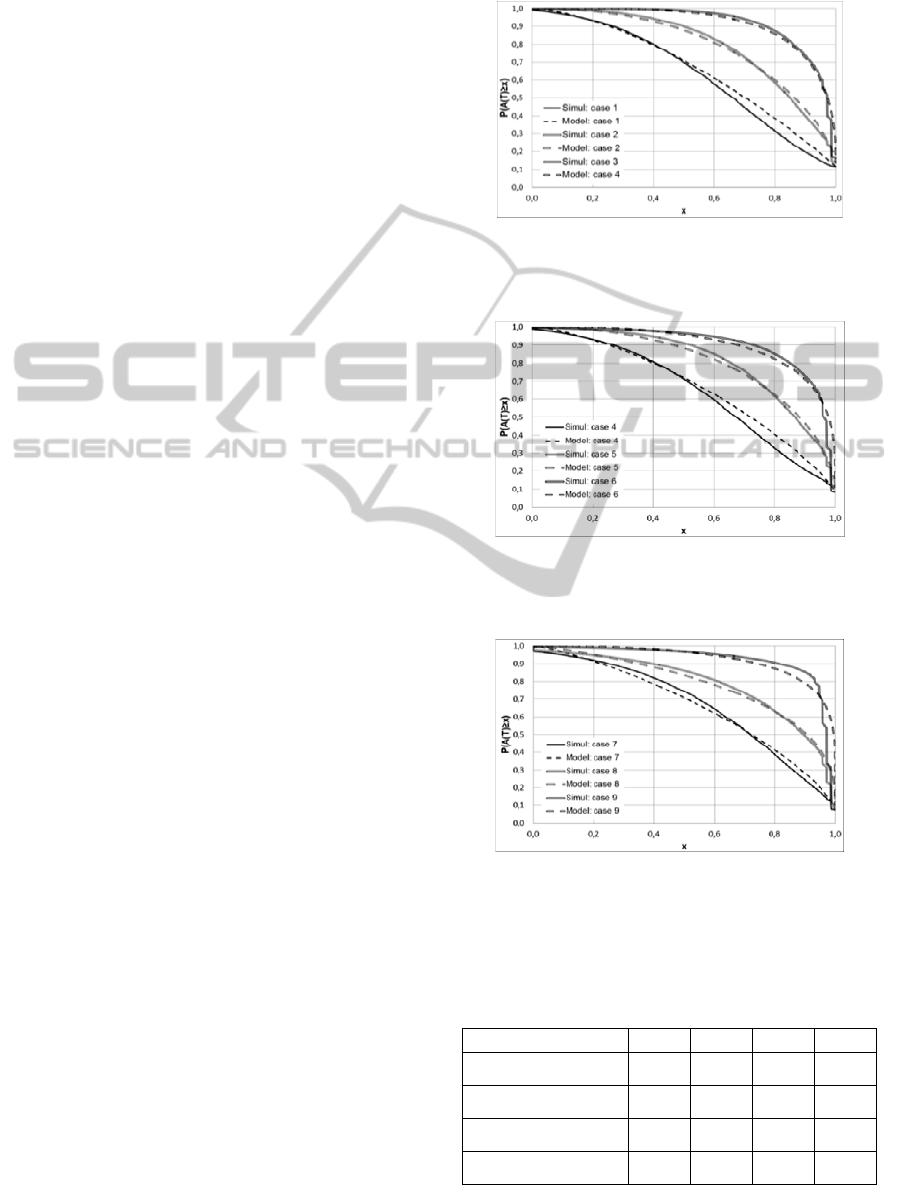
In Figure 3, 4 and 5, we show the survival

function of the interval availability using our model

and the simulation with M=10, 30, 50, respectively.

Note that the discontinuity points in the tail of A(T)

using simulation are due to the deterministic

assumption of the order-and-ship time. Observe that

our model has the highest accuracy for the cases

where M=10 and 30 and where E[A(T)] is larger

than 80%. Our model predicts very well E[A(T)] for

all the cases, see the second row in Table 1, and 2

for details. However, our model predicts Var[A(T)]

with less accuracy. Moreover, it seems that the

accuracy of Var[A(T)] has less impact on the

survival function than the accuracy of E[A(T)], see

for example the results of cases 3, 6, and 9. Note that

for all the different cases considered the difference

of (

(



)

≥), with ≥

[



(



)]

, obtained using

the simulation and our model is larger than -0.04 and

smaller than 0.07, as indicated in Table 1, and 2.

Finally, note that the run time of our approximation

is less 100ms for the considered cases.

Figure 2: Interval availability survival function with M=10

in case: 1. E[A(T)] = 63%, 2. E[A(T)] = 79%, and 3.

E[A(T)] = 92%.

Figure 3: Interval availability survival function with M=30

in case: 4. E[A(T)] = 64%, 5. E[A(T)] = 81%, and 6.

E[A(T)] = 90%.

Figure 4: Interval availability survival function with M=50

in case: 7. E[A(T)] = 66%, 8. E[A(T)] = 79%, and 9.

E[A(T)] = 92%.

Table 1: Relative absolute difference of E[A(T)] (resp.,

Var[A(T)]) obtained using our model and simulation for

case 1,2, 3, and 4.

Case

1 2 3 4

Relative absolute

difference E[A] (%)

3.68 0.17 0.35 3,67

Relative absolute

difference Var[A(T)] (%)

8.08 12.42 20.45 7,39

Min difference of

P(A(T)>x), x<=E[A(T)]

-0.04 -0.01 0 -0,04

Max difference

P(A(T)>x), x<=E[A(T)]

0.01 0.02 0.02 0,01

INTERVAL AVAILABILITY ANALYSIS OF A TWO-ECHELON, MULTI-ITEM SYSTEM

347

Table 2: Relative absolute difference of E[A(T)] (resp.,

Var[A(T)]) obtained using our model and simulation for

case 5, 6, 7,8 and 9.

Case

5 6 7 8 9

Relative absolute

difference E[A] (%)

0,49 0,11 0,34 0,17 0,22

Relative absolute

difference

Var[A(T)] (%)

12,83 7,01 6,77 4,22 1,51

Min difference of

P(A(T)>x),

x<=E[A(T)]

-0,01 -0,01 -0,03 -0,02 -0.01

Max difference

P(A(T)>x),

x<=E[A(T)]

0,03 0,03 0,04 0,03 0.07

6 CONCLUSIONS

In this paper we analyzed the interval availability of

a two-echelon network that supports multi-item

systems. We proposed an analytical approximation

that is based on a Markov chain analysis. We

computed in closed and exact form the expected, the

variance, and the probability of hundred percent

interval availability of the system. Using the

previous metrics we approximate the survival

function of the interval availability. The simulation

result shows that our model has accurate results

especially for high expected interval availability.

ACKNOWLEDGEMENTS

This research is part of ProSeLo project that is