
A WEARABLE GAIT ANALYSIS SYSTEM USING INERTIAL
SENSORS PART I
Evaluation of Measures of Gait Symmetry and Normality against 3D Kinematic
Data
A. Sant’Anna
1
, N. Wickstr
¨
om
1
R. Z
¨
ugner
2
and R. Tranberg
2
1
Intelligent Systems Lab, Halmstad University, Halmstad, Sweden
2
Department of Orthopedics, Sahlgrenska Academy, University of Gothenburg, Gothenburg, Sweden
Keywords:
Gait Analysis, Inertial Sensors, Symmetry, Normality.
Abstract:
Gait analysis (GA) is an important tool in the assessment of several physical and cognitive conditions. The lack
of simple and economically viable quantitative GA systems has hindered the routine clinical use of GA in many
areas. As a result, patients may be receiving sub-optimal treatment. The present study introduces and evaluates
measures of gait symmetry and gait normality calculated from inertial sensor data. These indices support the
creation of mobile, cheap and easy to use quantitative GA systems. The proposed method was compared to
measures of symmetry and normality derived from 3D kinematic data. Results show that the proposed method
is well correlated to the kinematic analysis in both symmetry (r=0.84, p<0.0001) and normality (r=0.81,
p<0.0001). In addition, the proposed indices can be used to classify normal from abnormal gait.
1 INTRODUCTION
Quantitative gait analysis (GA) can improve the as-
sessment of a number of physical and cognitive con-
ditions. The importance of GA in the treatment of
children with cerebral palsy is well known and doc-
umented, e.g. (Chang et al., 2010), (DeLuca et al.,
1997). The use of GA to monitor and assess Parkin-
son’s Disease, e.g. (Salarian et al., 2004), (Frenkel-
Toledo et al., 2005), and stroke, e.g. (Cruz et al.,
2008), (Silver et al., 2000), have also been investi-
gated. Changes in gait speed, gait variability, and neu-
rologic gait abnormalities have been associated with
the risk of developing dementia and mild cognitive
impairment, e.g. (Beauchet et al., 2008), (Verghese
et al., 2002).
Although the usefulness of GA is recognized by
the medical community, e.g. (Chang et al., 2010),
routine clinical use of GA is still not a reality. This
is likely due to the costs involved in performing a full
3D GA at a gait lab. As a result of not undergoing GA,
many patients may receive sub-optimal treatment, e.g.
(Kay et al., 2000), (Lofterød and Terjesen, 2008).
The simpler alternative to in-lab 3D GA is ob-
servational GA (OGA), such as the Gillette Func-
tional Assessment Questionnaire (GFAQ) Walking
Scale (Novacheck et al., 2000) and the Edinburgh Gait
Score (Read et al., 2003). Although some OGA meth-
ods have been shown valid and reliable, it is generally
understood that they are specific to patient groups,
subjective, and sensitive to the observer’s experience
(Toro et al., 2003). In 1999, Coutts (Coutts, 1999) ar-
gued that despite its limitations, OGA would never be
totally replaced as the default GA method in the clini-
cal environment because of ease of use. Current tech-
nological advancements, however, should encourage
clinicians to re-evaluate instrumented GA.
The goal of the present study is to develop a mo-
bile, cheap, and easy to use GA system that quantita-
tively evaluates certain characteristics of gait indepen-
dent of location and/or infrastructure. Such a system
may be complementary to 3D GA, by providing con-
tinuous or frequent monitoring. Alternatively, it may
be used where 3D GA is not available such as in un-
derprivileged areas or at home. The system may also
be coupled to OGA, providing consistent and reliable
quantitative data to aid clinical evaluation.
The proposed method uses accelerometer and gy-
roscope data to derive measures of gait symmetry
and gait normality. The signal analysis is based on
the symbolic approach presented in (Sant’Anna and
Wickstr
¨
om, 2010), and (Sant’Anna et al., 2011). 19
180
Sant’Anna A., Wickstrom N., Zügner R. and Tranberg R..
A WEARABLE GAIT ANALYSIS SYSTEM USING INERTIAL SENSORS PART I - Evaluation of Measures of Gait Symmetry and Normality against 3D
Kinematic Data.
DOI: 10.5220/0003707601800188
In Proceedings of the International Conference on Bio-inspired Systems and Signal Processing (BIOSIGNALS-2012), pages 180-188
ISBN: 978-989-8425-89-8
Copyright
c
2012 SCITEPRESS (Science and Technology Publications, Lda.)

healthy subjects were measured simultaneously with
inertial sensors and a 3D motion capture (MOCAP)
system while walking in different ways. Results from
the inertial system are compared to measures of sym-
metry and normality derived from 3D kinematic data.
2 RELATED WORK
2.1 Symmetry
Symmetry refers to the similarity between the move-
ments of the right and left sides of the body. Gener-
ally speaking, gait symmetry can be computed from
discrete values, e.g. spatio-temporal parameters; or
from continuous signals, e.g. joint angles. Some au-
thors have argued that discrete values are not always
sufficient to describe gait asymmetry, and that it is im-
portant to take into account continuous motion data
(Crenshaw and Richards, 2006). It is also important
to distinguish between different sources of data. In
the present study we will focus on kinematic data ex-
tracted from a MOCAP system; and accelerometer
and gyroscope data obtained via wearable sensors.
Some approaches to calculating symmetry using
continuous accelerometer data have been introduced.
(Moe-Nilssen and Helbostad, 2004), for example, in-
troduced an unbiased autocorrelation method using
trunk acceleration data. Although this may provide
a good general estimate of gait symmetry, it lacks in-
formation about each individual limb. More recently
(Gouwanda and Senanayake, 2011) used gyroscopes
on shanks and thighs to calculate symmetry using a
normalized cross correlation approach and the nor-
malized mean error between curves derived from right
and left sides. This method segments and normal-
izes the data to individual strides. As a result, only
the shape of the signal and not its relative temporal
characteristics are taken into account. Sant’Anna et
al. also suggested a symbolic method for estimating
gait symmetry using accelerometers (Sant’Anna and
Wickstr
¨
om, 2010) or gyroscopes (Sant’Anna et al.,
2011), which takes into account not only the shape
but also the temporal characteristics of the signal.
Kinematic gait data is usually evaluated by visual
inspection of superimposed curves from right and left
sides. Few symmetry measures have been proposed
which take into account complete joint angle curves.
(Crenshaw and Richards, 2006) calculated a measure
of trend symmetry based on the variance around the
1
st
principal component of a right-side vs. left-side
plot. This trend symmetry measure is insensitive to
scaling, and an additional measure, the range ampli-
tude ratio, is required. The present study introduces
a symmetry measure based on kinematic data which
can be expressed as one index.
2.2 Normality
Normality refers to the similarity between the move-
ments of one individual compared to average move-
ments of a population that is judged healthy/normal.
The Gillette Functional Assessment Questionnaire
(GFAQ) Walking Scale is a widely accepted gait nor-
mality measure based on observation. Considerable
efforts have been put into deriving a similar measure
from kinematic data. (Schutte et al., 2000) used prin-
cipal component analysis (PCA) on 16 discrete nor-
mal gait variables to create a representation of the data
in a different space. The magnitude of the projec-
tion of an abnormal data set onto this space is used
as a normality index, known as the Gillette Gait In-
dex (GGI). (Shin et al., 2010) used the same PCA ap-
proach to create three separate indices using variables
related to ankle, knee and hip kinematics.
A very similar PCA approach, the Gait Deviation
Index (GDI), was introduced by (Schwartz and Rozu-
malski, 2008) using complete joint angle curves. This
index showed high correlation with GGI, and distin-
guished between different levels of the GFAQ. One
advantage of PCA approaches is that they transform
the possibly dependent gait variables into a new set
of independent variables. The disadvantage is that re-
sults cannot be traced back to the original gait vari-
ables.
(Barton et al., 2007) used self organizing maps
(SOM) to create a single representation from many
kinetic and kinematic curves. This representation is
then used to calculate a measure of distance between
abnormal and normal data sets. This approach was
later developed into a user friendly graphical user in-
terface that provides a deviation curve for each sub-
ject (Barton et al., 2010). The mean value of this de-
viation curve was highly correlated with the GDI and
showed significant difference between different lev-
els of the GFAQ. The difficulty in using this method
derives from the fact that large amounts of normal ref-
erence data are needed to train the SOM.
A much simpler method, the Gait Profile Score
(GPS) and Movement Analysis Profile (MAP), was
introduced by (Baker et al., 2009). The MAP is cre-
ated by taking the root mean square error (RMS) be-
tween a reference joint angle curve and the corre-
sponding curve from a subject. This creates one nor-
mality index for each joint angle curve. A unique
index, the GPI, can be derived by concatenating all
joint angle curves end to end, and taking the RMS of
this aggregated curve. This work concluded that the
A WEARABLE GAIT ANALYSIS SYSTEM USING INERTIAL SENSORS PART I - Evaluation of Measures of Gait
Symmetry and Normality against 3D Kinematic Data
181

GPI and GDI are alternative and closely related mea-
sures. Although GDI presents some nice properties
such as normal distributions across GFAQ levels, GPS
is more easily interpreted because the original vari-
ables suffer no transformations and results are given
in degrees. (Beynon et al., 2010) also concluded that
GPS is significantly correlated with clinical judgment.
No normality indices based on accelerometer or
gyroscope data were found in the literature.
3 METHOD
3.1 Data collection
A group of 19 healthy individuals willing to partici-
pate in the experiment were randomly selected. The
average hight of the group was 172.1 ± 7.6 cm; and
the average weight was 71.8 ± 17.2 Kg. Seven par-
ticipants were male and twelve female, averaging an
age of 34 ± 13 years.
Kinematic and kinetic data were recorded with a
3D motion capture (MOCAP) system, Qualisys MCU
240, sampling at 240Hz. A total of 15 spherical re-
flective markers, of 19 mm in diameter, were attached
to the skin with double-sided tape. Markers were
placed on the sacrum, anterior superior iliac spine, lat-
eral knee-joint line, proximal to the superior border of
the patella, tibial tubercle, heel, lateral malleolus and
between the second and third metatarsals (Tranberg
et al., 2011).
Subjects were also equipped with 3 Shimmer
R
sensor nodes containing one 3-axis accelerometer and
one 3-axis gyroscope, sampling at 128Hz. The sen-
sor nodes were attached to the skin with double-sided
tape. One node was placed on each outer shank, about
3cm above the lateral malleolus marker, Figure 1(a).
The remaining node was placed mid-way between the
anterior superior iliac spine markers, Figure 1(b). In
addition, one reflective marker was also placed on
each sensor node.
(a) Shank sensor node (b) Waist sensor node
Figure 1: Placement of sensor nodes. Shank sensor node
approximately 3cm above the lateral malleolus reflective
marker, and waist sensor node mid-way between the ante-
rior superior iliac spine reflective markers.
Before starting the measurements, each sensor
node received a beacon signal from a host computer
with the host global time in milliseconds since epoch.
At this moment, each node stored in its memory card
its own local time in milliseconds since epoch to-
gether with the host global time. These records were
later used to synchronize the sensor data. The data
from the sensors is stored in the node.
The subjects were then asked to enter into the
measurement volume and a static reference record-
ing was obtained with the Mocap system while the
subjects were standing in an upright position aligned
with the x-axis of the global coordinate system. Prior
to recording, all subjects had the possibility to get fa-
miliarized with the walkway and define a comfortable
walking speed. The following instructions were then
given to the subjects: 1) walk normally at a comfort-
able speed; 2) walk with a limp, as if injured; and 3)
walk slowly, as if tired or pretending to be old. All
subjects performed three tests for each type of walk.
One test of each type was then randomly chosen for
further analysis.
This study was approved by the Regional Ethics
Board in Gothenburg, Sweden.
3.2 MOCAP Normality Measure
The normality index used for the kinematic data was
the GPS and the MAP (Baker et al., 2009). However,
the mean value was removed from all curves before
calculating the score, and foot progression was not
used because it was not available in the reference data
set. Removing the curves’ mean values makes the
normalcy measure more robust to offset errors, while
preserving the shape and range of the curves.
The reference data set is an ensemble of 34 ran-
domly selected adult subjects presenting no known
pathologies, previously acquired at the clinical gait
lab at Sahlgrenska University Hospital, Gothenburg,
Sweden. Joint angle curves were calculated for each
individual and normalized to stride time. The ensem-
ble average of the normalized curves was used as a
reference curve.
Each MAP component was calculated as the RMS
difference, MAP =
q
1
N
∑
N
n=1
(C
sub j
(n) −C
re f
(n))
2
,
between the reference curve, C
re f
, and the subject’s
curve, C
sub j
, Figure 2, where N is the number of
points in the curve. The GPS was calculated similarly
by concatenating all joint curves end to end.
For each subject, MAP and GPS results were cal-
culated as the average between right side and left side
MAP and GPS respectively.
BIOSIGNALS 2012 - International Conference on Bio-inspired Systems and Signal Processing
182
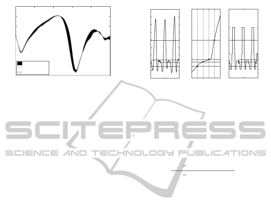
0 20 40 60 80 100
-20
-15
-10
-5
0
5
10
15
stride time (%)
normalized ankle df. angle (degrees)
difference
Subject's data
Reference data
Figure 2: Calculating the MAP. The MAP for this joint
angle progression is calculated as the RMS of the difference
between the subject’s curve and the reference curve, i.e. the
RMS of the shaded area.
3.3 MOCAP Symmetry Measure
Based on the GPS, a measure of symmetry was de-
rived for the kinematic data. In this case, the compo-
nents of MAP-symmetry were calculated as the RMS
error between the curves for the right and left sides,
after removing their corresponding mean values. Sim-
ilarly, GPS-symmetry was calculated by concatenat-
ing all joint curves end to end and calculating the
RMS difference between left and right sides.
3.4 Inertial Sensor Symmetry Measure
The symmetry measure used in this paper was pre-
sented in (Sant’Anna and Wickstr
¨
om, 2010) and also
used in (Sant’Anna et al., 2011), with a different sym-
bolization technique. The sensor signal, accelerom-
eter or gyroscope, is standardized to zero mean and
unitary standard deviation, then segmented into N
symbols. Symbolization is done by quantization into
N levels. The quantization levels are chosen based on
the empirical probability distribution of the signal, so
as to produce equiprobable symbols, Figure 3.
The period between consecutive occurrences of
the same symbol are calculated and stored in a period
histogram (Sant’Anna et al., 2011). Similarly, the pe-
riod between consecutive transitions from symbol i to
symbol j are calculated and stored in a transition his-
togram. The symmetry index is a measure of the sim-
ilarity between symbol (transition) period histograms
for the right and left sides. Histograms are compared
using a relative error measure shown in Eq. 1, where
Z is the number of symbols; K is the number of bins
in the histograms; n
i
is the number of non-empty his-
togram bins (for either foot) for symbol i; h
Ri
(k) is
the normalized value for bin k in the period histogram
i for the right foot; and h
Li
(k) is the normalized value
100 300 500
-1.5
-1
-0.5
0
0.5
1
1.5
2
2.5
3
time (samples)
standardized signal
A) original signal
0 0.2 0.4 0.6 0.8 1
-0.74
-0.46
-0.30
0.96
B) quantization
cumulative distr.
cut points
100 300 500
A
B
C
D
E
time (samples)
symbols
C) symbolized signal
Figure 3: Symbolization. In this example, the signal was
symbolized into 5 symbols. (A) shows the original signal
after standardization. (B) shows the empirical cumulative
distribution of the signal, probability levels are shown on
the horizontal axis. The quantization levels, cut points, are
the values at which the probability of the signal increases
by 1/Number
symbols
= 1/5 = 0.2. (C) illustrates the cor-
responding symbolized signal. Note that the probability of
each symbol occurring in the symbolized signal is 20%.
for bin k in the period histogram i for the left foot.
SI
symb
=
∑
Z
i=1
1
n
i
∑
K
k=1
|h
Ri
(k) −h
Li
(k)|
∑
Z
i=1
1
n
i
∑
K
k=1
|h
Ri
(k) +h
Li
(k)|
100 (1)
3.5 Inertial Sensor Normality Measure
The normality measure for the inertial sensor data was
derived from the symmetry measure, Part 3.4. In-
stead of comparing the histograms for right and left
sides, one subject’s histograms are compared to his-
tograms derived from a reference data set. The ref-
erence data set was formed by selecting the subjects
that presented the smallest GPS based on the normal
walk kinematic data.
The normal walk inertial sensor data from these
reference subjects was standardized to zero mean and
unitary standard deviation, symbolized, and symbol
(transition) periods were calculated. The symbol
(transition) periods were normalized to stride time.
That is, a period that coincides with stride time is
represented as 1 and all other periods are scaled cor-
respondingly. This normalization is common when
dealing with kinematic data, and it ensures that the
analysis is not affected by gait speed. The symbol
(transition) periods from all reference subjects were
used to create reference histograms.
Reference histograms were compared to the his-
tograms from right and left sides of each subject,
Eq. 2, where h
re f
are the reference histograms and
h
sub j
are the subject histograms. Right and left results
were averaged to create the normality measure for the
A WEARABLE GAIT ANALYSIS SYSTEM USING INERTIAL SENSORS PART I - Evaluation of Measures of Gait
Symmetry and Normality against 3D Kinematic Data
183
subject.
NORM
symb
=
∑
Z
i=1
1
n
i
∑
K
k=1
|h
re f
(k) −h
sub j
(k)|
∑
Z
i=1
1
n
i
∑
K
k=1
|h
re f
(k) +h
sub j
(k)|
100 (2)
3.6 Stride Time Estimation
The period (transition) histograms can also be used
to estimate gait events (Sant’Anna and Wickstr
¨
om,
2010). In the present study, stride time was calcu-
lated by first determining which of the symbols (tran-
sitions) presented periods with standard deviations
smaller or equal to 1/5 of their mean value. This rule
identifies the symbols (transitions) that occur regu-
larly in every cycle. The mean period of the high-
est symbol (transition) was used as an estimate of
the stride time. The highest symbol (transition) was
chosen based on a priori knowledge that the gyro-
scope data presents a prominent spike at mid-swing
(Salarian et al., 2004), and the accelerometer data
presents a prominent spike at heel-strike (Aminian
et al., 1999). As described in (Sant’Anna and Wick-
str
¨
om, 2010), a priori expert knowledge can be used
to identify gait events in the signal, from which vari-
ous temporal parameters may be derived, e.g. double-
support time.
3.7 Analysis
The data acquired from the MOCAP system was pro-
cessed in Visual 3D (C-Motion Inc., Germantown,
MD) to generate kinematic join angle data and spatio-
temporal parameters such as stride time. The data
was then exported to MATLAB (MathWorks, Natick,
MA) where MAP, GPS and MOCAP symmetry were
calculated for each subject and used as reference.
The signals from the shank accelerometers and
gyroscopes were low-pass filtered with a Butterworth
filter of order 6 and cut-off frequency 20Hz. The waist
sensor data was filtered at 10Hz. The signals were fil-
tered once, then reversed and filtered again to avoid
any phase shift. The three axes of each accelerometer
were combined into a resultant signal, A
res
=
q
A
2
x
+ A
2
y
+ A
2
z
.
For each gyroscope, only pitch and roll rotations were
considered, G
res
=
q
G
2
pitch
+ G
2
roll
.
Symmetry and stride times were calculated using
right and left shank signals. Normality was calcu-
lated using both shanks and waist signals. Measures
were calculated considering both period histograms
and transition histograms, varying from 5 to 25 sym-
bols. The resulting values outside two standard de-
viations were considered outliers and removed. The
remaining values were used to calculate the Spear-
man’s rank correlation coefficient with reference mea-
surements. The optimal number of symbols and the
choice of histogram were chosen so as to maximize
the correlation coefficients. A two-sample t-test was
used to determine if the final normality and symmetry
values distinguish between normal and other walks.
All hypothesis were bi-directional with confidence
level, α = 0.05. All sensor data analysis was under-
taken in MATLAB.
4 RESULTS
Some of the data was excluded due marker obstruc-
tion or sensor failure. The total number of subjects
used for each analysis is shown in Table 1.
Table 1: Number of subjects available for analysis.
walk placement accelerometer gyroscope
Normal
shank 16 14
waist 16 15
Slow
shank 13 12
waist 13 12
Limp
shank 16 14
waist 16 15
An example of the shank sensor node data and cor-
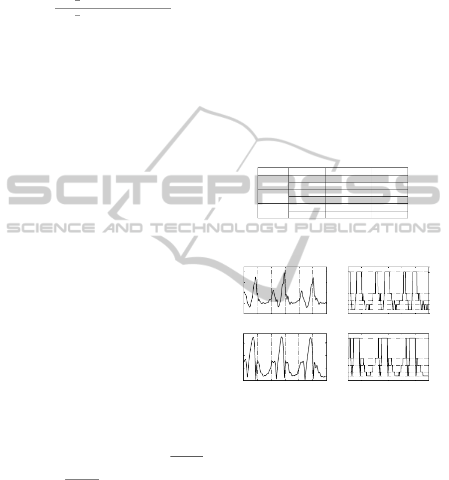
responding symbolized data is shown in Figure 4.
1.5 2 2.5 3 3.5 4 4.5
0
1
2
3
4
time (s)
acceleration (g)
A) resultant acceleration - right shank
1.5 2 2.5 3 3.5 4 4.5
A
B
C
D
E
time (s)
symbols
B) symbolized acceleration
1.5 2 2.5 3 3.5 4 4.5
0
2
4
6
time (s)
angular velocity (deg/s)
C) resultant angular velocity - right shank
1.5 2 2.5 3 3.5 4 4.5
A
B
C
D
E
time (s)
symbols
D) symbolized angular velocity
Figure 4: Example shank inertial sensor data. (A) illus-
trates a typical resultant acceleration signal from a shank
sensor. (B) exemplifies the symbolization of the acceler-
ation signal using 5 symbols. (C) illustrates a typical gy-
roscope resultant signal acquired with the same sensor as
(A). (D) exemplifies the symbolized gyroscope signal using
5 symbols. Signals (A) and (C) come from a normal walk
trial and are synchronized in time.
Figure 5 shows the MAP and GPS results for all
subjects during normal walking and limp walking.
There is a significant difference between the different
walks. The overall amplitude of the scores is reduced
by approximately a factor of 2 compared to results
presented (Baker et al., 2009). This is caused by the
absence of curves’ mean values. Another contribut-
ing factor is that the present work considers healthy
adults instead of children.
BIOSIGNALS 2012 - International Conference on Bio-inspired Systems and Signal Processing
184

ankle flex knee flex hip flex hip add hip rot pelv tilt pelv obliq pelv rot GPS
0
2
4
6
8
10
12
14
16
18
RMS error (degrees)
MAP: Normal walk vs. Limp walk
limp left side
limp right side
limp both sides
normal
Figure 5: MOCAP normality. MAP and GPS results for
the limp data set are shown against the normal data set re-
sults.
The best normality results using the shank sensors
were obtained with the accelerometer data, 5 sym-
bols, and symbol period histograms. Statistically sig-
nificant Spearman’s rank correlation coefficients are
shown in Table 2. Note that the normality measure
derived from the shank sensor correlates better with
ankle, knee and hip flexion MAP components than
with the other MAP components. The combination of
all MAP components into the GPS, however, corre-
lates better than most individual components, with the
exception of hip flexion. The normality index derived
from the accelerometer placed on the waist correlated
with the MOCAP reference better than the shank sen-
sor data, Table 3. The optimal combination in this
case was 18 symbols and transition histograms.
Table 2: Correlation of normality measures - shank.
sensor accelerometer
placement shank
histogram symbol period
no. symbols 5
variable r p-value
MAP ankle flex. 0.58 <0.0001
MAP knee flex. 0.73 <0.0001
MAP hip flex. 0.78 <0.0001
MAP pelv. obliq. 0.44 < 0.0001
MAP pelv. rot. 0.49 < 0.0001
GPS 0.74 < 0.0001
Table 3: Correlation of normality measures - waist.
sensor accelerometer
placement waist
histogram transition
no. symbols 18
variable r p-value
MAP ankle flex. 0.69 <0.0001
MAP knee flex. 0.77 <0.0001
MAP hip flex. 0.82 <0.0001
MAP hip add. 0.47 <0.0001
MAP pelv. obliq. 0.49 <0.0001
MAP pelv. rot. 0.71 < 0.0001
GPS 0.81 < 0.0001
The best correlation of the inertial sensor symme-
try with the reference was achieved with the shank gy-
roscopes, 20 symbols, and symbol period histograms.
The best correlation coefficients are shown in Table 4.
Once again, the measure derived from the shank sen-
sor correlates better with ankle, knee and hip flexion
MAP components.
Table 4: Correlation of symmetry measures - shank.
sensor gyroscope
placement shank
histogram symbol period
no. symbols 20
variable r p-value
ankle flex. 0.64 < 0.0001
knee flex. 0.81 < 0.0001
hip flex. 0.68 < 0.0001
all 0.84 < 0.0001
Stride time derived from the symbolized data were
accurate. The correlation with the reference data was
0.97, p<0.0001. After eliminating 2 outliers, the total
RMS error was 0.048 seconds. The best stride time
results were achieved using 17 symbols and transition
histograms.
Figures 6 and 7 show the symmetry and normal-
ity results respectively. Two-sample t-tests indicated
that the MOCAP symmetry data for normal walk was
significantly different from limp, p<0.0001, and slow
walk, p=0.03. The gyroscope symmetry index was
also significantly different between normal and limp,
p<0.0001, and normal and slow, p=0.02, data sets.
Similarly, normality indices were all significantly dif-
ferent between data sets, p<0.0001.
normal limp slow
1
2
3
4
5
6
7
8
9
10
11
12
MOCAP symmetry
A)
normal limp slow
10
20
30
40
50
60
70
shank gyroscope symmetry
B)
Figure 6: Symmetry indices. Distributions are presented
as boxplots. (A) illustrates the MOCAP symmetry results
for normal, limp and slow data sets. Results for the normal
data set were significantly different from limp (p<0.0001)
and slow (p=0.03) data sets. (B) shows the shank gyroscope
symmetry index, using 20 symbols and period histograms.
The symmetry of the normal data set was significantly dif-
ferent to that of limp (p<0.0001) and slow (p=0.02) data
sets.
5 DISCUSSION
It is important to stress that the MOCAP system
and the inertial sensors measure very different things.
Nonetheless, the raw data from both system can be
A WEARABLE GAIT ANALYSIS SYSTEM USING INERTIAL SENSORS PART I - Evaluation of Measures of Gait
Symmetry and Normality against 3D Kinematic Data
185

normal limp slow
1
2
3
4
5
6
7
8
9
10
11
12
13
MOCAP normality - GPS
A)
normal limp slow
50
55
60
65
70
75
80
85
90
95
100
waist accelerometer normality
B)
normal limp slow
10
15
20
25
30
35
40
45
50
shank accelerometer normality
C)
Figure 7: Normality indices. Distributions are presented
as boxplots. (A) shows the GPS for all three types of
walk. Normal and limp, and normal and slow data sets
were significantly different (p<0.0001). (B) illustrates the
normality results of all types of walk using the waist ac-
celerometer, 18 symbols, and transition histograms. Data
sets were significantly different (p<0.0001). (C) shows re-
sults of the normality index using shank accelerometers, 5
symbols, and symbol period histograms. Similarly, normal
walk was significantly different from limp and slow data
sets (p<0.0001).
processed in order to determine certain properties or
characteristics of gait which are the same or com-
parable. The MAP components, for example, con-
vey the normality of very specific joint movements.
The normality measure derived from the sensors, on
the other hand, expresses an overall normality of the
shank movements, which are caused by a combination
of different joint movements. The comparison of the
sensor normality with the different MAP components,
however, may provide insight into the the factors that
influence the sensor normality measure.
Although the shank sensor normality correlates
well with hip flexion and not with pelvic rotation, the
waist sensor normality correlates well with both. This
suggests that the shank sensors are mostly affected
by the abnormalities in hip flexion, whereas the waist
sensor is affected by abnormalities in hip flexion and
pelvic rotation. This is aligned with the fact most gait
pathologies affect the movement of the center of grav-
ity (Detrembleur et al., 2000), which is captured by
the waist sensor.
Another interesting factor is that the correlation
of sensor symmetry with the MOCAP symmetry con-
sidering all components, is greater than the correla-
tion with any individual component. This may sug-
gest that the symmetry of individual joint angles is not
representative of the symmetry of the movement as a
whole, or at least not representative of the movement
of the shanks. It is the combination of joint move-
ments that results in the overall symmetry captured
by the shank sensors.
One may argue that the lack of information about
individual joint movements or other particular kine-
matic and kinetic parameters diminishes the useful-
ness of the proposed method. However, the sym-
bolic representation, once it is properly understood,
may reveal more precise information about the move-
ment. Consider for example the signals shown in Fig-
ure 8. (A) illustrates the gyroscope resultant signal af-
ter symbolization of a subject walking normally, and
(B) shows the signal from the same sensor when the
subject was limping. Only two strides are depicted in
each plot.
Note how symbol D in the normal signal is re-
placed by signal C in the limp signal. It is known
that symbol C represents a lower angular velocity
than symbol D. As previously mentioned, it is also
known that these symbols occur shortly after heel-
strike. Therefore, this difference from normal to
limp indicates that the shank rotated more slowly af-
ter heel-strike when the subject was limping. Given
that the duration of the symbols is approximately the
same, the shank rotated to smaller angle. The extrac-
tion of such information is not trivial, but expert sys-
tems can be developed for this purpose. Another ad-
vantage of the proposed instrumented GA is that, after
a diagnosis or clinical evaluation has been made, the
recovery or progress of the patient can be easily mea-
sured according to symmetry and normality.
1.5 2 2.5 3
A
B
C
D
E
A) Normal walk - right shank gyroscope
time (s)
symbols
1 1.5 2 2.5
A
B
C
D
E
B) Limp walk - right shank gyroscope
time (s)
symbols
Figure 8: Comparing normal and limp walk. (A) illustrates
the gyroscope resultant signal after symbolization of a sub-
ject walking normally, and (B) shows the signal from the
same sensor when the subject was limping. Only two strides
are depicted in each plot. Note how symbol D in the normal
signal is replaced by signal C in the limp signal. This exem-
plifies how the symbolic representation of the signals may
be used to derive particular information about the subject’s
gait pattern.
Results show that the normal walk can be distin-
guished from the other walks with respect to normal-
ity and symmetry. Although limp and slow walk were
“acted” and not real, the purpose of the instructions
was to generate abnormal gait patterns. The distribu-
tion of the GPS shows that the fake patterns ranged
over varying levels of abnormality. This variety in the
BIOSIGNALS 2012 - International Conference on Bio-inspired Systems and Signal Processing
186

data is useful in evaluating the expressiveness of the
proposed method, and how well it covers a wide range
of abnormalities. Results suggest that the normality
and symmetry measures are gradual and can, in fact,
be used to express varying levels of abnormality.
One important observation is that the proposed
method utilizes several steps for the analysis. In con-
trast, the MOCAP system is commonly limited to
one stride per foot, because only two force plates are
available in most gait labs. The acquisition of a larger
number of steps greatly increases the amount of work
needed. Moreover, one stride may not be represen-
tative of a subject’s average gait pattern due to intra-
subject variability (Chau et al., 2005). The sensor data
used in the present study was relatively short, aver-
aging approximately 3 strides at constant speed for
normal and limp walk. Longer data recordings might
provide more accurate analysis.
When using inertial sensors for human movement
analysis, the placement of the sensors can greatly af-
fect results. In the present study, for example, the
waist sensor was attached to the front of the subject.
Most studies however, attach the sensor to the back,
e.g. (Moe-Nilssen and Helbostad, 2004), (Auvinet
et al., 1999), (Hartmann et al., 2009). The present
study is part of a larger study where hip-replacement
patients were being monitored with an inertial sensor
node for long periods of time. It was decided that a
sensor placed in the front would be more comfortable
than one in the back. The gait data collection kept the
same configuration. However, for short data collec-
tions, dealing with a varied pool of subject, it might
be beneficial to place the sensor at the back. This way,
the sensor may stay closer to the center of gravity re-
gardless of the weight or shape of the subject.
MOCAP systems and inertial sensor systems
should not compete, they should complement each
other. MOCAP systems measure the position of sets
of reflective skin markers, specific to a marker model
that defines the orientation of each body segment. Ac-
celerations, rotations and joint angles are obtained
through specific algorithms developed for that par-
ticular marker model. One may wonder if the con-
straints imposed by different models and filters distort
the original data. Gait is already a well studied area,
but new movements require new models. Inertial sen-
sors such as accelerometers and gyroscopes may con-
tribute to the study of movements that are not yet fully
understood, e.g. freezing of gait in Parkinson’s Dis-
ease patients (Plotnik et al., 2005), (Hausdorff et al.,
2003). They also complement MOCAP systems in
that they are mobile, and can be used in a wider vari-
ety of contexts.
6 CONCLUSIONS
This study presented and evaluated a method for gait
analysis using inertial sensor data. A novel method
for measuring gait normality was introduced, based
on a symbolic approach previously used for gait sym-
metry. Symmetry and normality results were com-
pared to a reference derived from kinematic data. Re-
sults support that an estimate of gait symmetry and
normality, related to that derived from MOCAP data,
can be obtained with a simple combination of inertial
sensors. This supports the development of a cheap
and easy to use system for quantitative gait analysis
that can be used both in the clinic and in other less
controlled environments.
The proposed measures of symmetry and normal-
ity correlate well with the reference GPS and sym-
metry MOCAP measures. A follow-up study on hip-
replacement patients will attempt to determine if the
proposed method is also in agreement with clinical
judgment. This expectation is supported by the fact
that GPS is, in turn, well correlated with clinical judg-
ment.
ACKNOWLEDGMENTS
This study was partially funded by the Promobilia
Foundation and the Institute of Health and Care Sci-
ences, Sahlgrenska Academy, University of Gothen-
burg, Sweden.
REFERENCES
Aminian, K., Rezakhanlou, K., De Andres, E., Fritsch, C.,
Leyvraz, P. F., and Robert, P. (1999). Temporal feature
estimation during walking using miniature accelerom-
eters: an analysis of gait improvement after hip arthro-
plasty. Medical and Biological Engineering and Com-
puting, 37:686–691.
Auvinet, B., Chaleil, D., and Barrey, E. (1999). Accelero-
metric gait analysis for use in hospital outpatients. Re-
vue du Rhumatisme: English ed., 66(7-9):389–397.
Baker, R., McGinley, J. L., Schwartz, M. H., Beynon,
S., Rozumalski, A., Graham, H. K., and Tirosh, O.
(2009). The gait profile score and movement analysis
profile. Gait & Posture, 30(3):265–269.
Barton, G., Lisboa, P., Lees, A., and Attfield, S. (2007).
Gait quality assessment using self-organising artificial
neural networks. Gait & Posture, 25(3):374 – 379.
Barton, G. J., Hawken, M. B., Scott, M. A., and Schwartz,
M. H. (2010). Movement deviation profile: A measure
of distance from normality using a self-organizing
neural network. Human Movement Science, In Press,
Corrected Proof.
A WEARABLE GAIT ANALYSIS SYSTEM USING INERTIAL SENSORS PART I - Evaluation of Measures of Gait
Symmetry and Normality against 3D Kinematic Data
187

Beauchet, O., Allali, G., Berrut, G., Hommet, C., Dubost,
V., and Assal, F. (2008). Gait analysis in demented
subjects: interests and perspectives. Neuropsychiatric
Disease and Treatment, 4(1):155–160.
Beynon, S., McGinley, J. L., Dobson, F., and Baker, R.
(2010). Correlations of the gait profile score and the
movement analysis profile relative to clinical judg-
ments. Gait & Posture, 32(1):129–132.
Chang, F. M., Rhodes, J. T., Flynn, K. M., and Carollo,
J. J. (2010). The role of gait analysis in treating gait
abnormalities in cerebral palsy. Orthopedic Clinics of
North America, 41(4):489 – 506.
Chau, T., Young, S., and Redekop, S. (2005). Manag-
ing variability in the summary and comparison of gait
data. Journal of NeuroEngineering and Rehabilita-
tion, 2(1):22.
Coutts, F. (1999). Gait analysis in the therapeutic environ-
ment. Manual Therapy, 4(1):2 – 10.
Crenshaw, S. J. and Richards, J. G. (2006). A method for
analyzing joint symmetry and normalcy, with an ap-
plication to analyzing gait. Gait & Posture, 24(4):515
– 521.
Cruz, H. et al. (2008). Evidence of abnormal lower-limb
torque coupling after stroke: An isometric study sup-
plemental materials and methods. Stroke, 39(1):139.
DeLuca, P. A., Davis, R. B., unpuu, S., Rose, S., and
Sirkin, R. (1997). Alterations in surgical decision
making in patients with cerebral palsy based on three-
dimensional gait analysis. Journal of Pediatric Or-
thopaedics, 17(5):608–614.
Detrembleur, C., van den Hecke, A., and Dierick, F. (2000).
Motion of the body centre of gravity as a summary
indicator of the mechanics of human pathological gait.
Gait & Posture, 12(3):243–250.
Frenkel-Toledo, S., Giladi, N., Peretz, C., Herman, T., Gru-
endlinger, L., and Hausdorff, J. (2005). Effect of gait
speed on gait rhythmicity in Parkinson’s disease: vari-
ability of stride time and swing time respond differ-
ently. Journal of NeuroEngineering and Rehabilita-
tion, 2(1):23.
Gouwanda, D. and Senanayake, A. S. M. N. (2011). Iden-
tifying gait asymmetry using gyroscopes–a cross-
correlation and normalized symmetry index approach.
Journal of Biomechanics, 44(5):972 – 978.
Hartmann, A., Murer, K., de Bie, R., and de Bruin, E. D.
(2009). Reproducibility of spatio-temporal gait pa-
rameters under different conditions in older adults us-
ing a trunk tri-axial accelerometer system. Gait &
Posture, 30(3):351–355.
Hausdorff, J. M., Schaafsma, J. D., Balash, Y., Bartels,
A. L., Gurevich, T., and Giladi, N. (2003). Impaired
regulation of stride variability in parkinson’s disease
subjects with freezing of gait. Experimental Brain Re-
search, 149:187–194.
Kay, R. M., Dennis, S., Rethlefsen, S., Reynolds, R. K.,
Skaggs, D. L., and Tolo, V. T. (2000). The effect
of preoperative gait analysis on orthopaedic decision
making. Clinical Orthopaedics and Related Research,
372:217–222.
Lofterød, B. and Terjesen, T. (2008). Results of treatment
when orthopaedic surgeons follow gait-analysis rec-
ommendations in children with cp. Developmental
Medicine & Child Neurology, 50(7):503–509.
Moe-Nilssen, R. and Helbostad, J. L. (2004). Estimation
of gait cycle characteristics by trunk accelerometry.
Journal of Biomechanics, 37(1):121 – 126.
Novacheck, T. F., Stout, J. L., and Tervo, R. (2000). Re-
liability and validity of the gillette functional assess-
ment questionnaire as an outcome measure in chil-
dren with walking disabilities. Journal of Pediatric
Orthopaedics, 20(1):75.
Plotnik, M., Giladi, N., Balash, Y., Peretz, C., and Haus-
dorff, J. M. (2005). Is freezing of gait in Parkinson’s
disease related to asymmetric motor function? Annals
of Neurology, 57(5):656–663.
Read, H. S., Hazlewood, M. E., Hillman, S. J., Prescott,
R. J., and Robb, J. E. (2003). Edinburgh visual gait
score for use in cerebral palsy. Journal of Pediatric
Orthopaedics, 23(3):296–301.
Salarian, A., Russmann, H., Vingerhoets, F., Dehollain, C.,
Blanc, Y., Burkhard, P., and Aminian, K. (2004). Gait
assessment in Parkinson’s disease: Toward an ambula-
tory system for long-term monitoring. IEEE Transac-
tions on Biomedical Engineering, 51(8):1434 –1443.
Sant’Anna, A., Salarian, A., and Wickstr
¨
om, N. (2011). A
new measure of movement symmetry in early parkin-
son’s disease patients using symbolic processing of in-
ertial sensor data. IEEE Transaction on biomedical
Engineering. Epub ahead of print, 2011.
Sant’Anna, A. and Wickstr
¨
om, N. (2010). A symbol-based
approach to gait analysis from acceleration signals:
Identification and detection of gait events and a new
measure of gait symmetry. IEEE Transactions on In-
formation Technology in Biomedicine, 14(5):1180 –
1187.
Schutte, L. M., Narayanan, U., Stout, J. L., Selber, P., Gage,
J. R., and Schwartz, M. H. (2000). An index for quan-
tifying deviations from normal gait. Gait & Posture,
11(1):25–31.
Schwartz, M. H. and Rozumalski, A. (2008). The gait de-
viation index: A new comprehensive index of gait
pathology. Gait & Posture, 28(3):351–357.
Shin, K.-Y., Rim, Y., Kim, Y., Kim, H., Han, J., Choi, C.,
Lee, K., and Mun, J. (2010). A joint normalcy index
to evaluate patients with gait pathologies in the func-
tional aspects of joint mobility. Journal of Mechanical
Science and Technology, 24:1901–1909.
Silver, K., Macko, R., Forrester, L., Goldberg, A., and
Smith, G. (2000). Effects of aerobic treadmill train-
ing on gait velocity, cadence, and gait symmetry in
chronic hemiparetic stroke: A preliminary report.
Neurorehabilitation and Neural Repair, 14(1):65–71.
Toro, B., Nester, C., and Farren, P. (2003). A review of ob-
servational gait assessment in clinical practice. Phys-
iotherapy Theory and Practice, 19(3):137–149.
Tranberg, R., Saari, T., Z
¨
ugner, R., and K
¨
arrholm, J. (2011).
Simultaneous measurements of knee motion using an
optical tracking system and radiostereometric analysis
(RSA). Acta Orthopaedica, 82(2):171–176.
Verghese, J., Lipton, R., Hall, C., Kuslansky, G., Katz, M.,
and Buschke, H. (2002). Abnormality of gait as a
predictor of non-Alzheimer’s dementia. New England
Journal of Medicine, 347(22):1761.
BIOSIGNALS 2012 - International Conference on Bio-inspired Systems and Signal Processing
188
