ESTIMATING PLANAR STRUCTURE IN SINGLE IMAGES
BY LEARNING FROM EXAMPLES
Osian Haines and Andrew Calway
University of Bristol, Bristol, U.K.
Keywords:
Monocular vision, Image understanding, Single image, Plane detection, Planar structure, Scene analysis,
Learning, Nearest neighbour, Topic discovery, Latent semantic analysis, Spatiogram.
Abstract:
Outdoor urban scenes typically contain many planar surfaces, which are useful for tasks such as scene re-
construction, object recognition, and navigation, especially when only a single image is available. In such
situations the lack of 3D information makes finding planes difficult; but motivated by how humans use their
prior knowledge to interpret new scenes with ease, we develop a method which learns from a set of train-
ing examples, in order to identify planar image regions and estimate their orientation. Because it does not
rely explicitly on rectangular structures or the assumption of a ‘Manhattan world’, our method can generalise
to a variety of outdoor environments. From only one image, our method reliably distinguishes planes from
non-planes, and estimates their orientation accurately; this is fast and efficient, with application to a real-time
system in mind.
1 INTRODUCTION
We address the problem of detecting planes in a sin-
gle image, and estimating their 3D orientation. Man-
made environments tend to contain many planes, and
these can be used for compact representation of 3D
scenes (Bartoli, 2007) and more efficient robot navi-
gation (Gee et al., 2008; Mart
´
ınez-Carranza and Cal-
way, 2010). The ability to discover planes from only
a single image would be beneficial in tasks includ-
ing image understanding (Saxena et al., 2008), recon-
structing 3D models (Ko
ˇ
seck
´
a and Zhang, 2005) or
wide baseline matching (Mi
ˇ
cu
ˇ
s
´
ık et al., 2008).
Finding planes in single images is challenging,
due to the of lack of depth information. One popu-
lar approach is to use vanishing lines (Ko
ˇ
seck
´
a and
Zhang, 2005) to infer the scene geometry; however,
this presupposes that such structure exists. Our ap-
proach (figure 1) is instead motivated by humans’ ap-
parent ability to understand scenes from one view: we
learn from the appearance of a set of examples, man-
ually labelled with their class and orientation; and de-
scribe these with feature descriptors in a bag of words,
enhanced with spatial information. Using these train-
ing images allows us to identify image regions as pla-
nar – for building fac¸ades, stone walls and so on –
or as non-planar – for foliage, vehicles, etc; then for
planar regions we estimate their 3D orientation.
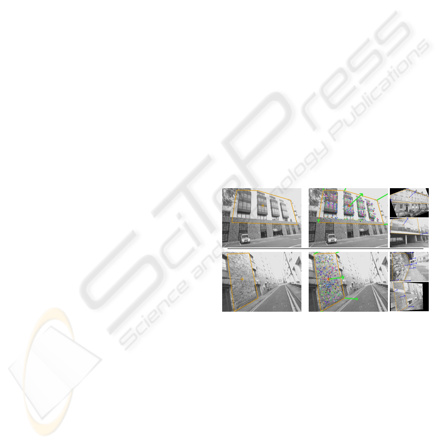
Figure 1: For a given image region (left) our algorithm clas-
sifies them as planes and estimates their orientation (cen-
tre) by finding training examples with similar orientation
(right).
The method accurately separates planes from non-
planes, making a sufficiently confident decision in
91% of cases, with 90% accuracy; plane orientation is
predicted with a mean error of around 14° . Since we
do not rely on vanishing lines or rectangular structure,
the method is applicable to a wider range of scenes.
The method is fast, able to make a decision for a new
region in under one second. In this work we consider
only the classification and orientation of individual
image regions – automatic detection or segmentation
is left for future work.
289
Haines O. and Calway A. (2012).
ESTIMATING PLANAR STRUCTURE IN SINGLE IMAGES BY LEARNING FROM EXAMPLES.
In Proceedings of the 1st International Conference on Pattern Recognition Applications and Methods, pages 289-294
DOI: 10.5220/0003708902890294
Copyright
c
SciTePress

The paper is organised as follows. Section 2 dis-
cusses related work, then section 3 describes the de-
tails of the method. The results in section 4 show that
the method can distinguish planes from non-planes
and reliably predict their orientation in a variety of
situations, and we conclude in section 5 with sugges-
tions for future work.
2 RELATED WORK
A standard way to obtain geometry from a single
image is the use of vanishing points – for example
(Ko
ˇ
seck
´
a and Zhang, 2005) rely on the orthogonality
of planes to group lines and hypothesise rectangles,
from which the pose of the camera can be recovered.
Similarly, (Mi
ˇ
cu
ˇ
s
´
ık et al., 2008) treat rectangle de-
tection as a labelling problem, and use the detected
planes’ orientation for wide baseline matching.
Another cue which may be exploited is the dis-
tinctive appearance of certain parts of images. The
method most similar to our own is that of (Hoiem
et al., 2007), which classifies ‘super-pixels’ into ge-
ometric classes, with orientations limited to being ei-
ther horizontal, left, right, or front facing. A vari-
ety of features are used to create a coherent grouping
from the initial super-pixels, resulting in an esimate
of scene layout which has been used to create simple
3D models and for object recognition.
(Saxena et al., 2008) focus on the related task of
estimating depth, by training on range data from a
laser scanner. From absolute and relative depth esti-
mates at individual regions, a Markov Random Field
is used to find a consistent depth map over the whole
image. This has been used for sophisticated 3D model
building, and to drive a high-speed toy car (Michels
et al., 2005).
These methods show considerable progress in un-
derstanding single images; however they either rely
on a restrictive ‘Manhattan’ assumption, or when ap-
plicable to more general scenes, can only obtain very
coarse orientation or depth.
3 METHOD
Here we give an overview of our method, with more
details in subsequent subsections. First, we gather a
database of training examples, and manually assign
a class (plane or not plane) and orientation (normal
vector). Then the class and orientation of new regions
are estimated using a K-Nearest Neighbour classifier,
with similarity between regions evaluated as follows.
(a) (b) (c)
(d) (e) (f)
Figure 2: Examples of the training data we use, showing
the manually selected region of interest and plane orienta-
tion (regions (a)-(d)); examples (d) and (f) were obtained by
warping the original images.
We use histograms of oriented gradients to de-
scribe the local appearance at salient points in an im-
age region; since these are not informative enough on
their own, we accumulate information using a bag of
words approach, applying a variant of Latent Seman-
tic Analysis (Deerwester et al., 1990) for dimension-
ality reduction.
The resulting vectors of latent ‘topics’ can be used
for classification and orientation, but performance is
improved by also considering their spatial configu-
ration, which we represent using a histogram aug-
mented with means and covariances – a ‘spatiogram’
(Birchfield and Rangarajan, 2005); as far as we are
aware, using a spatiogram with a bag of words is
novel. Further technical details can be found in
(Haines and Calway, 2011).
3.1 Training Data
We collect training images of planes and non-planes
from a variety of outdoor locations; these have a res-
olution of 320 × 240 pixels, and have been corrected
for radial distortion. For each image we mark a re-
gion of interest, and assign them to the plane or non-
plane class as appropriate. To get the true orientation,
corners of a quadrilateral are marked, corresponding
to a real rectangle; this defines two orthogonal sets
of parallel lines, whose intersections define vanishing
points v
1
and v
2
. From this we calculate n, the normal
vector of the plane, using n = K
T
l, where l = v
1
× v
2
is the vanshing line of the plane and K is the 3 × 3
matrix encoding the camera paramters (see figure 2).
We generate more training examples, to approx-
imate planes seen from different viewpoints, by ap-
plying geometric transformations to the images. The
simplest of these is to reflect about the vertical axis;
we can also use the known relative pose of the planar
regions to render new views from different locations,
ICPRAM 2012 - International Conference on Pattern Recognition Applications and Methods
290

via the homography H = R + tn
T
/d, where R and t
are the rotation matrix and translation vector for the
new view, and d is the perpendicular distance to the
plane (defined up to scale). H is used to warp the im-
age, to approximate the plane as seen from the new
viewpoint, while the normal vector is rotated by R. In
practice, the range of possible warps is limited by the
image resolution.
3.2 Features
Following more typical object recognition ap-
proaches, we use descriptors that describe local ori-
entations, in a histogram of oriented gradients. While
this is the basis descriptors like SIFT (Lowe, 2004),
we emphasise that our task is quite different: one of
the benefits of SIFT is that it is invariant to a wide
range of deformations, whereas our aim is specifically
to determine plane orientation, not identity.
For each patch, we create gradient histograms for
each quadrant, each with 12 angular bins, and con-
catenate these to form a descriptor of 48 dimensions
– this is to capture some local structure information
and build a richer descriptor.
Feature descriptors are created at salient points in
the image, detected using the Difference of Gaussians
detector (DoG), which gives a location and scale for
each point. We use the scale to set the width of the
patch to create the descriptor; scale selection seems to
be advantageous since it ensures the most appropriate
scale is being used at each location – this is verified
by our results (see section 4), which show that multi-
scale DoG detection is consistently superior to both
single-scale DoG and FAST (Rosten and Drummond,
2006).
3.3 Bag of Words
The gradient descriptors capture information about
local areas, but are not sufficient to disambiguate the
structure of the scene, so we accumulate information
over the whole region using the bag of words model.
Each image region is represented by a histogram x
over N words (typically N = 300; see section 4); term
frequency - inverse document frequency weighting is
used to down-weight common words, resulting in the
weighted word vector x
0
.
The words are found by quantising each of the D
descriptor vectors d
d
in the image region to a code-
book; the codebook is built by clustering descriptors
extracted from a set of typical images, using K-means
with N cluster centres.
3.3.1 Topic Discovery
When N is large, the word vector will be high dimen-
sional and sparse, and encodes no relationship bew-
teen potentially synonymous words. We overcome
this using Orthogonal Nonnegative Matrix Factorisa-
tion (ONMF) to reduce the word histogram to a vec-
tor of latent topic weights. ONMF is related to Latent
Semantic Analysis (LSA) (Deerwester et al., 1990),
but differs in that the topic vectors have non-negative
components (this is essential, see section 3.4).
ONMF factorises the term-document matrix X
(where X
n j
is the (weighted) number of occurrences
of word n in image j, for M images) into X ≈ WH,
where W is the basis of the latent topic space (of rank
T , the number of topics), and H contains the topic
vectors. Word vectors are approximated by x
0
i
≈ Wh
i
,
where h
i
is topic vector; conversely the topic vector
for a new word vector is h
i
= W
T
x
i
(because W is
orthogonal).
ONMF factorisation has no closed form solution,
so we use an iterative method (Choi, 2008) which
alternates the following updates (the columns of W
must be re-normalised after each iteration):
W
nt
←− W
nt
(XH
T
)
nt
(WHX
T
W)
nt
(1)
H
tm
←− H
tm
(W
T
X)
tm
(W
T
WH)
tm
(2)
3.4 Spatiograms
The constellation and star models (Fergus et al., 2005)
have shown that representing the spatial arrange-
ment of descriptors can improve performance; how-
ever because these are computationally expensive we
use spatiograms instead (Birchfield and Rangarajan,
2005). A spatiogram is a higher-order generalisation
of a histogram, where each bin also has a mean and
covariance matrix, summarising the points contribut-
ing to it. A spatiogram S
word
over the words consists
of a set of N triplets s
n
= hh
n
,µ
n
,Σ
n
i, were h
n
is the
bin count, µ
n
is the mean and Σ
n
the covariance ma-
trix of the 2D coordinates for points contributing to
the histogram bin. These are calculated as follows
(altered so that we can use them for words, weighted
words, or topics):
µ
n
=
1
α
D
∑
d=1
v
d
λ
dn
(3)
Σ
n
=
α
α
2
− β
D
∑
d=1
(v
d
− µ
n
)(v
d
− µ
n
)
T
λ
dn
(4)
ESTIMATING PLANAR STRUCTURE IN SINGLE IMAGES BY LEARNING FROM EXAMPLES
291
where v
d
is the 2D point at which descriptor d
d
is
created, and α =
∑
D
d=1
λ
dn
, β =
∑
D
d=1
λ
2
dn
. For the
basic word spatiogram, the element weight λ
dn
is
equal to 1 iff descriptor d quantises to word n; for
the spatiogram of weighted words S
word0
, λ
dn
=
x
0
n
x
n
,
i.e. the weighted occurrence of each word in the im-
age. The topic spatiogram S
topic
(of length T ) uses
λ
dt
=
x
0
n
x
n
W
nt
, where n is the word to which descriptor
d
d
quantises, and W
nt
is the component of the basis
vector for topic t relating to word n. Note that all
weights must be positive – the reason we use ONMF
instead of LSA. To compare spatiograms during clas-
sification we use the distance metric proposed by (
´
O
Conaire et al., 2007). As we show in section 4, in-
cluding spatial information boosts performance con-
siderably.
3.5 Classification
To classify image regions and estimate their orienta-
tion, we use the relatively simple K-Nearest Neigh-
bour classifier (KNN), chosen because analysing the
chosen neighbours (see figures 1, 5) allows us to ver-
ify the method works as expected. Classification and
orientation estimation can be performed simultane-
ously, by finding the K nearest neighbours: the class is
assigned to the majority class of these, and the orien-
tation is the mean of the 3D normal vectors. The pro-
portion of neighbours in the larger class can be used
as a confidence value to reject less certain classifica-
tions.
4 RESULTS
We collected an initial data set of 556 regions, from
an urban area. For evaluation we use five-fold cross
validation, and all tests use a value of K = 5 nearest
neighbours, chosen for its superior performance (ex-
periments omitted for brevity). First we analyse the
performance of using ONMF and spatiograms, com-
pared to the basic bag of words: we ran the algorithm
using the (weighted) word histograms x
0
only, on
word-spatiograms S
word0
, on topic vectors h only, and
on topic spatiograms S
topic
(the full method), for vary-
ing vocabulary size. Figure 3 shows results for classi-
fication accuracy and orientation error: in general, us-
ing topic discovery out-performs using words directly.
Performance using word histograms decreases as they
become sparser with increasing vocabulary size, but
topic vectors can extract meaningful information from
high dimensional word vectors, and performance re-
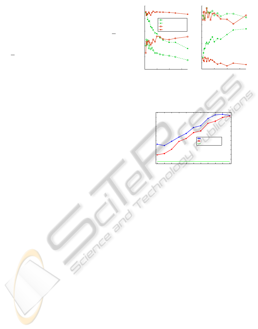
mains almost constant. The graphs also clearly show
0 200 400 600
0.65
0.7
0.75
0.8
0.85
0.9
Number of words
Classification accuracy
Word histogram
Word spatiogram
20−Topic histogram
20−Topic spatiogram
(a) Classification accuracy.
0 200 400 600
17
18
19
20
21
22
23
24
25
26
27
Number of words
Orientation error (degrees)
(b) Orientation error.
Figure 3: Comparison of words and topics for different vo-
cabulary sizes.
5 10 15 20 25 30 35 40 45 50 55
14
15
16
17
18
19
20
21
22
23
24
25
Patch width
Orientation error
FAST − single scale
DoG − single scale
DoG − scale selection
Figure 4: Using the Difference of Gaussians detector to
choose the scale at which descriptors are built outperforms
any single fixed scale, detected with either DoG or FAST.
the benefit of using spatiograms, which outperform
histograms in all cases.
Interestingly, the results suggest that a very small
number of words can be used without topic discov-
ery – however, this constrains the method to use
only small vocabularies, while are likely to generalise
poorly to new data sets. We verified this on our in-
dependent data set (see below) and found that in this
case, using words alone gave an orientation accuracy
of 20.5° (with standard deviation 18.1°), compared to
using topics with error of 17.5° (std 15.9°).
We also ran an experiment to verify that using
scale selection for the features is important. To en-
sure that no one scale was the best with scale selection
simply choosing this occasionally, we tested scale se-
lection (using the DoG detector) against fixed patch
sizes with widths from 5 to 55, detected with both
FAST and DoG; as figure 4 shows, scale selection is
always better than any one scale.
Finally, we augment the training set by reflecting
and warping regions (section 3.1), giving a total of
7752 (we do not test on the warped images, and en-
sure no region can match to a warped version of it-
self). This decreases the mean orientation error from
17.2° (standard deviation 13.7°) to 14.3° (std 12.9°).
ICPRAM 2012 - International Conference on Pattern Recognition Applications and Methods
292
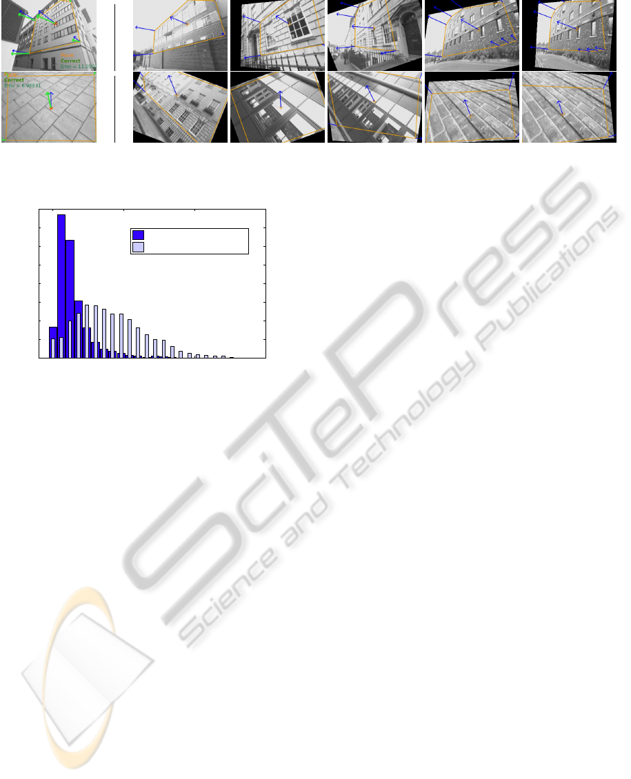
Figure 5: Examples of test planes (far left) and their 5 nearest neighbours. Top: matching to neighbours with different
appearance. Bottom: accurate orientation estimation, though there are no images of the ground in the training set.
0 50 100 150
0
200
400
600
800
1000
1200
1400
1600
Orientation error (degrees)
Our method
Random neighbours
Figure 6: Distribution of errors for our method (dark),
showing the majority of errors are small. Comparison to
random neighbours method is superimposed (light).
For the remaining tests we use DoG for feature po-
sition and scale selection, the full set of warped exam-
ples, topic spatiograms in a vocabulary of 300 words,
and we discard regions with a confidence below 0.7.
The results we obtain for this situation is a recall (per-
centage of regions above the confidence threshold) of
91%, classification accuracy of 90%, and a mean ori-
entation error of 14°. Figure 6 shows a histogram
for orientation estimation, clearly showing that for
the majority of regions (81%), the error is in the re-
gion of 0° to 20°. For comparison, and to indicate
what a mean error of 14° signifies, we show resuts
of an experiment using randomly chosen neighbours
(histogram overlayed on the same plot). Clearly our
method performs much better than chance – where
the mean error is above 40°; this is a useful validation
of the method, as it shows our method is not merely
exploiting an artefact of how the data are distributed.
4.1 Independent Data
We also tested the algorithm on an independent data
set collected from a different urban area, with the data
set from above used for training. We achieved similar
performance – a recall of 91%, classification accuracy
of 87%, and mean orientation error of 17.5°. This
set included some difficult regions – some without
the classic rectangular-structure appearance (figures
1,7(d)), as well as images of pavements and roads,
while we were careful to include no images of the
ground in the training set, to test generalisation (fig-
ures 5 bottom, 7(f),7(g)). Figure 5 shows some exam-
ple results of orientation estimation, alongside their
nearest neighbours: these are often quite different in
appearance, yet have a similar orientation. Figure
7 shows further examples, including non-planar re-
gions. In these images, blue (thin) arrows indicate
ground truth, and green (thicker) arrows are the esti-
mated normal, with cyan circles denoting non-planar
classification.
Figure 8 shows cases where the method performs
poorly, for example 8(a) and 8(b) where all the neigh-
bouring planes have very different orientation, a rare
situation which requires further investigation. Figure
8(d) is a more difficult example, since it is quite differ-
ent from any training images. Figure 8(e) may be con-
fused by the railings, vertical trees and strong horizon
line; and it is interesting to note that 8(f) is incorrectly
determined to be a plane, when the side of a van could
arguably be considered planar.
5 CONCLUSIONS
We have shown that we can reliably determine
whether regions of images are planar or not, and
estimate their orientation with respect to the view-
point. This is successfully achieved using information
from just one image in a bag of words representation,
where performance is improved by using latent topic
discovery and encoding spatial information. A KNN
classifier was sufficient to demonstrate that the algo-
rithm is able to classify a wide variety of plane and
non-plane images and accurately estimate plane ori-
entation (more advanced classifiers would be a nat-
ural aventue of future work); our method can work
even in examples devoid of typical structure such as
ESTIMATING PLANAR STRUCTURE IN SINGLE IMAGES BY LEARNING FROM EXAMPLES
293
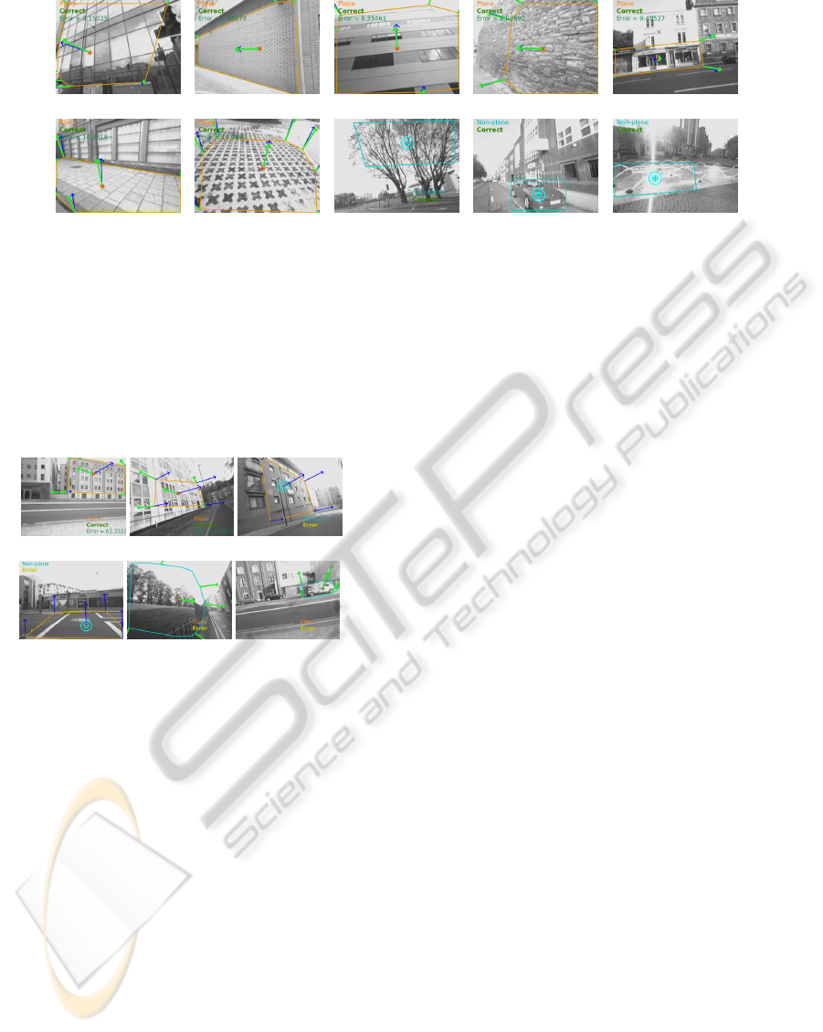
(a) (b) (c) (d) (e)
(f) (g) (h) (i) (j)
Figure 7: Examples of (a)-(g) planes with good orientation estimates and (h)-(j) correctly classified non-planes.
vanishing points and images of rectangles, and gen-
eralises well to new data. Now that we have shown
this is possible, we intend to develop our algorithm to
automatically segment planar regions from images –
since we operate on whole regions as opposed to us-
ing local colour or edge information this will require
a different approach to standard image segmentation.
(a) (b) (c)
(d) (e) (f)
Figure 8: Where the method fails: (a),(b) show planes with
incorrect orientation estimate, whereas (c),(d) are false neg-
atives and (e),(f) are false positives for plane classification.
ACKNOWLEDGEMENTS
This work was funded by UK EPSRC. With thanks to
Jos
´
e Mart
´
ınez-Carranza and Sion Hannuna for useful
discussions and advice.
REFERENCES
Bartoli, A. (2007). A random sampling strategy for piece-
wise planar scene segmentation. Computer Vision and
Image Understanding, 105(1).
Birchfield, S. and Rangarajan, S. (2005). Spatiograms ver-
sus histograms for region-based tracking. In Com-
puter Vision and Pattern Recognitionn, volume 2.
Choi, S. (2008). Algorithms for orthogonal nonnegative
matrix factorization. In International Joint Confer-
ence on Neural Networks. IEEE.
Deerwester, S., Dumais, S., Furnas, G., Landauer, T., and
Harshman, R. (1990). Indexing by latent semantic
analysis. Journal of the American society for Infor-
mation Science, 41(6).
Fergus, R., Perona, P., and Zisserman, A. (2005). A sparse
object category model for efficient learning and ex-
haustive recognition. In Computer Vision and Pattern
Recognition, volume 1.
Gee, A., Chekhlov, D., Calway, C., and Mayol-Cuevas, W.
(2008). Discovering higher level structure in visual
slam. Transactions on Robotics, 24.
Haines, O. and Calway, A. (2011). Estimating planar
structure in single images by learning from examples.
Technical Report CSTR-11-005, University of Bristol.
Hoiem, D., Efros, A., and Hebert, M. (2007). Recovering
surface layout from an image. International Journal
of Computer Vision, 75(1).
Ko
ˇ
seck
´
a, J. and Zhang, W. (2005). Extraction, match-
ing, and pose recovery based on dominant rectangular
structures. Computer Vision and Image Understand-
ing, 100(3).
Lowe, D. (2004). Distinctive image features from scale-
invariant keypoints. International Journal of Com-
puter Vision.
Mart
´
ınez-Carranza, J. and Calway, A. (2010). Unifying pla-
nar and point mapping in monocular slam. In British
Machine Vision Conference.
Michels, J., Saxena, A., and Ng, A. (2005). High speed
obstacle avoidance using monocular vision and rein-
forcement learning. In International Conference on
Machine learning.
Mi
ˇ
cu
ˇ
s
´
ık, B., Wildenauer, H., and Ko
ˇ
seck
´
a, J. (2008). De-
tection and matching of rectilinear structures. In Com-
puter Vision and Pattern Recognition.
´
O Conaire, C., O’Connor, N. E., and Smeaton, A. F. (2007).
An improved spatiogram similarity measure for robust
object localisation. In International Conference on
Acoustics, Speech and Signal Processing, volume 1.
Rosten, E. and Drummond, T. (2006). Machine learning for
high-speed corner detection. Lecture Notes in Com-
puter Science, 3951.
Saxena, A., Sun, M., and Ng, A. (2008). Make3d: learning
3d scene structure from a single still image. Transac-
tions on Pattern Analysis and Machine Intelligence.
ICPRAM 2012 - International Conference on Pattern Recognition Applications and Methods
294
