COMPARING LINEAR AND CONVEX RELAXATIONS FOR

STEREO AND MOTION

Thomas Schoenemann

Lund University, Lund, Sweden

University of Pisa, Pisa, Italia

Keywords:

Motion estimation, Convex relaxation.

Abstract:

We provide an analysis of several linear programming relaxations for the problems of stereo disparity estima-

tion and motion estimation. The problems are cast as integer linear programs and their relaxations are solved

approximately either by block coordinate descent (TRW-S and MPLP) or by smoothing and convex optimiza-

tion techniques. We include a comparison to graph cuts. Indeed, the best energies are obtained by combining

move-based algorithms and relaxation techniques. Our work includes a (slightly novel) tight relaxation for the

typical motion regularity term, where we apply a lifting technique and discuss two ways to solve the arising

task. We also give techniques to derive reliable lower bounds, an issue that is not obvious for primal relaxation

methods, and apply the technique of (Desmet et al., 1992) to a-priori exclude some of the labels. Moreover we

investigate techniques to solve linear and convex programming problems via accelerated ﬁrst order schemes

which are becoming more and more widespread in computer vision.

1 INTRODUCTION

First order methods for correspondence problems, in

particular stereo and motion, have received a lot of

attention over the past few years. The arising opti-

mization problems are largely solved today, and it is

time to compare the different techniques. In doing

so, we focus on a topic that has been widely ignored

for computer vision: in a primal relaxation scheme,

what can we truly conclude about the associated lower

bound? Most standard approaches require a very high

precision to give a guaranteed lower bound, which is

impractical.

The addressed models are discrete multi-label

problems and can be cast as Markov Random Fields

with binary terms. As unary data terms do not impose

algorithmical challenges we focus on the regularity

terms, considering ones that can be expressed in terms

of absolute differences of indicator functions: linear

potentials and the Potts model.

Subsequently, we consider two types of linear pro-

gramming relaxations: the standard marginal poly-

tope relaxation associated to inference in Markov

Random Fields, and specialized linear relaxations

where absolute differences are modeled by a con-

straint system. For the latter, we consider a simple

variant and a much tighter relaxation based on lifting.

The problem with these relaxations is that they are

convex, but neither strictly convex nor differentiable,

which makes solving them exactly very cost inten-

sive. In this paper we evaluate two common strategies

to deal with this problem: for the marginal polytope

relaxation we use block-coordinate descent methods

(Kolmogorov, 2006; Globerson and Jaakkola, 2007;

Sontag et al., 2010) that may not ﬁnd the exact relax-

ation value, but usually get very close to it.

For the specialized relaxations we consider

smoothing techniques that approximate the linear re-

laxations via strictly convex and differentiable func-

tions. These functions are convex relaxations of

the original discrete optimization problem. To solve

the smoothed problems, we apply optimization tech-

niques that are becoming increasingly popular in

Computer Vision but have not been applied to the ex-

act considered problems yet. A basic scheme con-

sists of combining accelerated ﬁrst order schemes

(Nesterov, 2004) with the projection on a product

of simplices (Michelot, 1986), plus a smoothing of

non-smooth functions (Nesterov, 2005). This scheme

has been used in (Lellmann et al., 2009; Goldl

ucke

and Cremers, 2010). In a second scheme, we apply

the well-known augmented Lagrangian method (Bert-

sekas, 1999, chap. 4.2) to the linear programming for-

mulations.

Previously (Szeliski et al., 2008), energy mini-

mization methods have been compared in a discrete

context including stereo, but excluding motion. In

contrast, we focus on correspondence problems and

Schoenemann T. (2012).

COMPARING LINEAR AND CONVEX RELAXATIONS FOR STEREO AND MOTION.

In Proceedings of the 1st International Conference on Pattern Recognition Applications and Methods, pages 5-14

DOI: 10.5220/0003710400050014

 SciTePress

lifting techniques. We start with a review of common

approaches for stereo and motion. The optimization

techniques underlying the most relevant works will be

reviewed in a later section.

Stereo. To get an overview of methods for

stereo disparity estimation, the taxonomy given in

(Scharstein and Szeliski, 2002) is still a very good

starting point. A quite robust approach that guaran-

tees global optima for certain ﬁrst-order priors was

given by (Ishikawa, 2003) and later formulated in

(Pock et al., 2008) as a continuous problem. (Bhus-

nurmath and Taylor, 2008) address second order pri-

ors via customized linear programming and a convex-

iﬁcation of the data term.

To further improve the robustness of these models,

typically non-convex regularization terms are used,

and the resulting optimization problems become hard.

(Kleinberg and Tardos, 1999) cast the Potts model as

a linear program, and (Zach et al., 2008) solve this

by coordinate descent on a modiﬁed functional. The

top-performing methods are currently based on belief

propagation (Klaus et al., 2006; Yang et al., 2009)

or the related tree reweighted message passing (Kol-

mogorov, 2006). (Meltzer et al., 2005) show how

to obtain global optima by running several stages of

these techniques.

Finally there are move-based algorithms like ex-

pansion moves (Boykov et al., 2001). In a less direct

approach, fusion moves have been considered (Wood-

ford et al., 2008).

Motion. We focus on non-parametric methods to

the estimation of optical ﬂow. Traditionally here one

minimizes a ﬂow-ﬁeld energy with a non-convex data

term and a convex regularizer. This trend was started

by (Horn and Schunck, 1981) and much reﬁned sub-

sequently. In particular, robust data terms and reg-

ularizers based on absolutes have been considered

(Memin and Perez, 1998; Papenberg et al., 2006).

Also, different optimization techniques have been ex-

plored (Papenberg et al., 2006; Bruhn, 2006; Zach

et al., 2007) and second order priors were considered

(Trobin et al., 2008). All of these methods rely on re-

peated convexiﬁcation of the energy. Some of them

are among the best performing known today.

In a more recent line of work, one instead works

with a discretized set of possible motion vectors.

One way to address the arising discrete optimization

problem is given by move-based algorithms (Boykov

et al., 2001; Glocker et al., 2008). The remaining

techniques can all be viewed as linear or convex pro-

gramming methods. (Shekhovtsov et al., 2008) in-

troduce a clever application of tree reweighted mes-

sage passing (Kolmogorov, 2006), where horizontal

and vertical displacements are separate variables.

(Goldstein et al., 2009) propose a lifting technique

to solve the non-linearized motion problem in terms

of indicator variables for level sets. Below, we give a

different solution with indicator variables for labels -

the advantage being that we only have easy-to-handle

simplex constraints.

Recently (Goldl

ucke and Cremers, 2010) pro-

posed a very memory efﬁcient technique for large

scale non-linearized motion estimation, using a con-

vexiﬁcation of non-convex terms. However, as we

show later in this work, the optimal energy is always

zero and the corresponding minimizers are meaning-

less. Hence, this method requires a careful initializa-

tion and must not be run until convergence.

2 THE PROBLEMS

In this paper we consider multi-label problems with

unary and binary terms, i.e. of the general form

E(y) =

∑

p∈V

) +

∑

(p,q)∈N

p,q

) (1)

where y : V → {1,...,L}, p,q denote locations de-

ﬁned by a set of points V ⊆ R

and N is a neigh-

borhood system, usually the 8-neighborhood in this

work. We require that N is asymmetric, i.e. if (p,q) ∈

N then (q, p) /∈ N . Further, it will be convenient to

abbreviate N (p) = {q |(p,q) ∈ N ∨ (q, p) ∈ N }.

2.1 Stereo

In stereo, one is given two images showing the same

scene and wants to ﬁnd out where the points in the

ﬁrst image are to be found in the second image. It is

known that each point can be found along a certain

epipolar line. For simplicity, in this work we assume

that these lines coincide with scan-lines in the image.

Given two images I

: Ω → R , where Ω ⊂ R

in a continuous formulation one is then searching for

a disparity map d : Ω → R that describes the displace-

ments. In our ﬁrst model, the optimal disparity map

is deﬁned as the optimum of

Ω

(x,y) − I

(x + d(x,y), y)|

dxdy

+ λ

Ω

|∇d(x,y)| dxdy ,

where p is some positive power and λ > 0 a weighting

factor. The ﬁrst term is the data term, and we simply

choose p = 1 in this work. The second term is called a

regularizer, and we will meet one other choice below.

ICPRAM 2012 - International Conference on Pattern Recognition Applications and Methods

Most current top-performing methods are based

on discretizing the continuous model and, more im-

portantly, the range of the function d. That is, we now

assume that d : V → L, where V is the set of pixel

locations and L ⊂ R is a ﬁnite set. For this work we

assume that the points in L are induced by an equidis-

tant spacing.

Instead of integrals, in the data term one is now

considering sums over the pixels in the image. Dis-

cretizing the regularity term is more intricate. We will

consider the approximation

|∇d(p)| ≈

∑

q∈N (p)

|d(p)− d(q)|

kp − qk

Methods derived from the continuous model will typ-

ically take a Euclidean vector norm of the gradient

here (Goldstein et al., 2009; Goldl

ucke and Cremers,

2010), known as total variation. By deﬁning

D(p = (x, y), l) = |I

(x,y) − I

(x + l,y)|

we are ﬁnally ready to phrase the ﬁrst discrete model

considered in this work:

∑

D(p,d(p)) + λ

∑

(p,q)∈N

|d(p)− d(q)|

kp − qk

. (SA)

For the second model we directly consider the discrete

formulation which amounts to the Potts model:

∑

D(p,d(p)) + λ

∑

(p,q)∈N

1 − δ(d(p),d(q))

kp − qk

, (SP)

where δ(·,·) is the Kronecker delta.

2.2 Motion

Motion is a generalization of stereo to arbitrary two-

dimensional displacements, denoted by two functions

u : Ω → R and v : Ω → R for the displacement in hori-

zontal and vertical direction, respectively. The contin-

uous formulation of the model we will consider looks

as follows:

Ω

(x,y) − I

(x + u(x,y),y + v(x,y))|dxdy

+ λ

Ω

|∇u(x,y)| + |∇v(x,y)|

dx dy .

Here, we have convex regularizers but a non-convex

data term which makes the problem difﬁcult. Re-

cently there has been increasing interest (Shekhovtsov

et al., 2008; Goldstein et al., 2009; Goldl

ucke and

Cremers, 2010) in methods that discretize the ranges

of the displacement functions. That is, we are now

considering u : V → L

and v : V → L

, where L

and L

are ﬁnite subsets of R . The discrete model

looks as follows:

∑

p∈V

(x,y) − I

(x + u(x,y),y + v(x,y))| (MA)

+λ





∑

(p,q)∈N

|u(p) − u(q)|

kp − qk

∑

(p,q)∈N

|v(p) − v(q)|

kp − qk





The resulting optimization problem is much harder

than (SA) for stereo. Since with a Potts potential it

would be even more difﬁcult, we will not consider a

variant (MP) here.

2.3 Why Lower Bounds?

Above two essential problems of computer vision

have been cast as energy minimization problems. In

practice it is desirable but not strictly necessary to ﬁnd

the global minimum of these problems: the functions

are designed in a way that any solution with energy

in a certain band around the optimal one should be an

acceptable solution. Hence, if one is able to provide

a tight lower bound, any method that ﬁnds a solution

close to this bound will give valuable insights into the

suitability of the models for relevant real-world in-

stances of the problem.

2.4 Excluding Labels

In the absence of a regularity term (i.e. λ = 0) the

above problems are easy to solve: the optimal label

can be determined independently for each pixel. As

soon as there is a regularity term, even with a very

small λ, this no longer works. However, with the help

of the dead-end elimination algorithm of (Desmet

et al., 1992) it is still possible to at least exclude some

of the labels. We state this (adapted to our context) in

the following proposition:

Proposition 1. Consider the general energy (1) and

assume V

p,q

(·,·) ≥ 0 everywhere. For any site p, pick

a k

∈ arg min

(l). Now, if for any label l

(l) > D

) +

∑

q:(p,q)∈N

max

p,q

,l) , (2)

then y

6= l in any optimal solution y.

Proof: Assume that y

∗

is an optimal solution satis-

fying y

∗

= l and denote its energy c

∗

. Now deﬁne

ˆy



if v = p

∗

else .

Then the cost of

y are

ˆc = c

∗

+ D

(k) − D

(l) +

∑

q∈N (p)

p,q

∗

) −V

p,q

(l,y

∗

)] .

COMPARING LINEAR AND CONVEX RELAXATIONS FOR STEREO AND MOTION

Exploiting the condition (2) on D

(l), it follows that

ˆc < c

∗

∑

q∈N (p)

p,q

∗

) − max

p,q

)

−V

p,q

(l,y

∗

)]

≤ c

∗

y has a lower energy than y

∗

. A contradiction. 

For (SP) up to 25% of all labels can be excluded,

and we exploit this information to initialize the con-

vex relaxation methods.

3 LINEAR PROGRAMMING

RELAXATIONS

In this paper, we evaluate strategies to solve the

problems (SA),(SP) and (MA) by ﬁrst casting them

as integer linear programs and then (approximately)

solving the arising linear programming relaxations.

Hence, we are dealing with constrained optimization.

All formulations are based on indicator functions to

express which pixel has which label.

For stereo, all considered methods introduce a bi-

nary variable x

∈ {0,1} for every p ∈ V and every

label d ∈ L, where a value of 1 indicates that y

= d.

The variables are grouped into a vector x

. Among

other things, the constraint system expresses that ev-

ery pixel must have exactly one label:

∈ S

∑

d∈L

ˆx

= 1 ∀p ∈ V

Together with the constraint x

≥ 0 that is naturally

satisﬁed for binary variables such a constraint system

is known as a product of simplices, an important fact

for several of the methods we consider below.

For motion, there are two different approaches. In

one of them there is a binary variable x

h,v

∈ {0,1} for

every pixel p ∈ V and combination of displacements

h ∈ L

,v ∈ L

. All these variables are grouped into

a vector x

H×V

. The constraint that every pixel have

exactly one label is now expressed as

H×V

∈ S

H×V

∑

h,v

ˆx

h,v

= 1 ∀p ∈ V

In the other approach there are separate binary

variables x

p,H

and x

p,V

for every pixel p ∈ V to ex-

press the horizontal and vertical displacements of a

pixel. They are grouped into a vector x

HkV

. Now ev-

ery pixel must have exactly one horizontal and exactly

one vertical label, expressed as

HkV

∈ S

HkV

∑

ˆx

p,H

∑

ˆx

p,V

=1 ∀p ∈ V

In both methods we again have products of simplices.

All of these problems are based on binary variables.

However, these often make the arising constrained op-

timization problems very hard. As a consequence,

x ∈ {0,1} is often relaxed to the constraint x ∈ [0,1]

and the resulting problem is in all considered cases a

linear programming relaxation (when using smooth-

ing this turns into a non-linear but still convex prob-

lem).

Before we proceed to present the considered

methods, we note that the data terms of (SA) and

(SP) can now be expressed as a linear function c

those for motion as a linear function c

H×V

where

= |I

(p) − I

(p + (d 0)

h,v

= |I

(p) − I

(p + (h v)

)| .

3.1 Marginal Polytope Formulations

All considered problems are inference problems for

Markov Random Fields with unary and pairwise

terms. There is a standard integer linear programming

formulation (and associated LP-relaxation) for such

problems, called the marginal polytope formulation.

Here we detail it by directly choosing (SA) and

(SP) as applications. Problem (1) is here re-phrased

as the integer linear program

min

∑

l∈L

(l) · z

∑

(p,q)∈N

∑

p,q

) · z

p,q

s.t.

∑

p,q

= z

∀p ∈ V ,l

∈ L (3)

∑

p,q

= z

∀q ∈ V ,l

∈ L

∈ {0, 1} ∀p ∈ V ,l ∈ L .

For general V

p,q

(·,·) this integer programming prob-

lem is NP-hard, so one aims at solving the linear

programming relaxation, i.e. relaxing z

∈ {0,1} to

∈ [0,1]. However, actually storing all pairwise vari-

ables z

p,q

is only practicable for a very small number

of labels and hence not applicable for stereo. Hence,

using a standard linear programming solver is not an

option here. Instead there are specialized block coor-

dinate descent algorithms which we introduce below.

Many of these methods have already been tested

on the problem of stereo, e.g. (Kolmogorov, 2006).

For motion we note the work of (Shekhovtsov et al.,

2008) who show how to efﬁciently solve the problem

(MA) with these techniques. They build on variables

HkV

, so there are no longer any unary terms: the

data term is now binary, too. This results in savings

in memory and run-time compared to the straightfor-

ward solution with variables x

H×V

ICPRAM 2012 - International Conference on Pattern Recognition Applications and Methods

3.2 Specialized Linear Programming

We now turn to specialized linear programming re-

laxations which take into account that the regularity

terms are functions of absolute differences, i.e. terms

of the form |y

− y

| where y

∈ L. At ﬁrst glance

this does not apply to the Potts model. However, as

exploited by (Kleinberg and Tardos, 1999; Zach et al.,

2008), the Potts model can be written as a sum of ab-

solute differences in terms of the indicator variables:

1 − δ(y

) =

∑

l∈L

− x

| . (4)

Finally, minimizing terms of the form |y

− y

| is

equivalent to the linear program (see e.g. (Dantzig and

Thapa, 1997))

min

p,q

−

p,q

+ a

p,q

−

(5)

s.t. y

− y

= a

p,q

− a

p,q

−

p,q

≥ 0, a

p,q

−

≥ 0 .

By itself this problem is trivial and the optimum 0.

However, this construction also holds when integrated

into larger linear programs (as e.g. derived below),

provided the auxiliary variables a

p,q

−

are not used

for other constraints.

While the Potts model (4) can now be directly

translated to a linear program, for (SA) and (MA)

this is more difﬁcult: the models here involve differ-

ences between labels, i.e. in terms of the variables y,

whereas it is often convenient to state the problem in

terms of the binary indicator variables x. Below we

detail two ways on the problem of stereo, then brieﬂy

discuss the transfer to motion estimation.

Simple Relaxations. A simple way, used in (Lell-

mann et al., 2009; Goldl

ucke and Cremers, 2010), to

express the absolute difference |y

− y

| in terms of

indicator variables is given by

− y

| =



∑

l∈L

l · (x

− x

)



While for binary variables this expression holds ex-

actly, we will see later that the associated relaxations

are quite weak. The linear program corresponding to

(SA) is now

min

x,a

∑

p,q∈N

kp − qk

p,q

+ a

p,q

−

]

s.t.

∑

l∈L

l · (x

− x

) = a

p,q

− a

p,q

−

∀(p,q) ∈ N ,

∈ S

≥ 0 , a

≥ 0 .

Relaxations based on Lifting. A technique that gives

much stronger relaxations is called lifting and was

used by (Ishikawa, 2003) to show that (SA) can be

globally optimized via graph cuts - the linear pro-

gramming relaxation is here equivalent to the integer

linear program. In the considered setting, lifting is

closely related to level sets, i.e. it can be expressed

using variables



1 if y

≤ l

0 else

∑

≤l

With these variables we can now express the original

absolute differences as sums of absolute differences

of the level variables:

− y

| =

∑

l∈L



− u



and obtain the linear program

min

x,a

∑

p,q∈N

kp − qk

p,q

+ a

p,q

−

]

s.t.

∑

≤l

− x

] = a

p,q

+,l

− a

p,q

−,l

∀(p,q) ∈ N ,l ∈ L,

∈ S

≥ 0 , a

≥ 0 .

Motion Relaxation. Both introduced techniques

can be transferred to the problem of motion estima-

tion when using the variables x

H×V

. For simplicity

we state the models in terms of absolute differences

and leave the construction

a la (5) to the reader. The

simple relaxation can be cast as

min

H×V

∑

(p,q)∈N

kp − qk



∑

h,v

v · [x

h,v

− x

h,v

]



∑

(p,q)∈N

kp − qk



∑

h,v

h · [x

h,v

− x

h,v

]



s.t. x

H×V

∈ S

H×V

, x

H×V

≥ 0 .

The lifted version is stated here as

min

H×V

∑

(p,q)∈N

kp − qk

∑

p,H

− u

q,H

∑

(p,q)∈N

kp − qk

∑

p,V

− u

q,V

s.t. u

p,H

= u

p,H

h−1

∑

h,v

p,V

= u

p,V

v−1

∑

h,v

H×V

∈ S

H×V

, x

H×V

≥ 0 .

Note that here it is straightforward to eliminate the

variables u as they are deﬁned by acyclic equality

constraints.

COMPARING LINEAR AND CONVEX RELAXATIONS FOR STEREO AND MOTION

3.3 Quadratic Programming

Formulations

Recently (Goldl

ucke and Cremers, 2010) proposed

to model problems with product label spaces such

as (MA) as a quadratic integer programming prob-

lem with an indeﬁnite cost function. They build on

the separate variable version x

HkV

and (in the discrete

analogon) express the cost function as

∑

p∈V

∑

h,v

· x

p,H

· x

p,V

These are sums of second order non-convex terms and

the authors propose to convexify the problem by re-

placing each term by its lower convex envelope:

∑

p∈V

∑

h,v

· max{0,x

p,H

+ x

p,V

− 1} . (6)

The maximization could again be translated to a linear

programming relaxation. This relaxation would nat-

urally ﬁt into our survey. However, we have already

stated in the introduction that it does not make sense,

and will now substantiate this:

Lemma 1. Suppose |L

| ≥ 3 and |L

| ≥ 3. Then the

minimal value of (6) s.t. x

HkV

∈ S

HkV

≥ 0 is 0.

Proof: Consider

p,H

= 1/|L

| ∀p ∈ V , h ∈ L

p,V

= 1/|L

| ∀p ∈ V , v ∈ L

Then x

p,H

+ x

p,V

≤ 2/3 and hence max{0,x

p,H

p,V

− 1} = 0 for all p ∈ V ,h ∈ L

,v ∈ L

. 

The given x

HkV

is identical for all pixels, and since a

typical regularization term for stereo and motion will

be at its minimum for such a conﬁguration, this is

the global minimum even for regularized functionals.

The solution is meaningless: it assigns equal proba-

bility to all possible labelings.

4 ALGORITHMS

There are standard software packages for (nearly) ex-

actly solving linear programming relaxations. How-

ever, in practice they do not scale well: e.g. (Meltzer

et al., 2005) found they could handle images of size

up to 39 × 39 for the marginal polytope relaxation in

stereo with 30 disparities.

For the specialized relaxations the situation is a bit

better: we solved the motion relaxation for a 75 × 75

image with displacements between −8 and 8 in steps

of 1 in both horizontal and vertical directions (= 289

labels) using a standard solver. This required roughly

3 GB and several hours computing time, so in practice

it is still too inefﬁcient.

Instead we consider approximate techniques to

solve the relaxations, either using block coordinate

descent or using smoothing techniques. In practice

these methods get very close to the actual relaxation

value.

4.1 The Marginal Polytope

A number of popular algorithms to (approximately)

solve the marginal polytope relaxations are based on

block coordinate descent on dual problem formula-

tions. Here we explore two of them.

TRW-S. (Wainwright et al., 2005) proposed an ap-

proach where the blocks of the dual take the form

of trees. One then alternates the estimation of min-

marginals in the trees (using the inward-outward al-

gorithm) with reparameterization steps. The origi-

nal formulation was not monotonically improving the

dual bound, but the issue was solved by TRW-S (Kol-

mogorov, 2006). We will later see that in practice this

methods gets very close to the optimum.

The running times per iteration are in general

quadratic in the number of labels. However, for

many kinds of potentials (e.g. Potts and absolute dif-

ferences) there are more efﬁcient ways to perform

inward-outward - see e.g. (Felzenszwalb and Hutten-

locher, 2006).

MPLP. Recently (Globerson and Jaakkola, 2007)

introduced a new message passing algorithm derived

from a non-standard dual of the marginal polytope al-

gorithm. On this formulation they perform block co-

ordinate descent where (for pairwise MRFs) a block

considers all dual variables associated to a particular

edge. See also (Sontag et al., 2010) for a very good

explanation and further background on the method.

The method is very efﬁcient and monotonically in-

creases the dual bound. It allows the same kind of

optimizations as TRW-S.

4.2 Specialized Relaxations

For the specialized relaxations we tried block coordi-

nate descent on the primal relaxation, using standard

LP-solvers. This resulted in heavily suboptimal so-

lutions and the running times were still too high. As

a consequence, for these problems we apply smooth-

ing techniques. Note that the smoothed problems are

themselves valid relaxations of the discrete optimiza-

tion problem: the cost for integral solutions are the

same as in the discrete problem.

ICPRAM 2012 - International Conference on Pattern Recognition Applications and Methods

Smoothing. (Nesterov, 2005) shows how a large

class of non-differentiable functions can be closely

approximated by differentiable functions with

Lipschitz-continuous gradients. Here, very efﬁcient

numerical schemes can be applied (Nesterov, 2004).

In our context, the employed approximation

|x| ≈



|x| −

if |x| ≥ ε

2ε

else

where ε > 0 is a small constant. We scale this func-

tion so that it gives exact values for x = ±1. This ex-

pression is substituted wherever absolutes occur in the

problem formulation. One obtains a convex function

to be optimized over a product of simplices, which is

done by combining (Nesterov, 2004) with the algo-

rithm (Michelot, 1986) to re-project on the simplices.

Augmented Lagrangians Instead of smoothing the

absolutes, one can work directly with the linear pro-

gram and apply the very general augmented La-

grangian method (Bertsekas, 1999, chap. 4.2), which

is applicable to many constrained optimization prob-

lems. Here we consider

min

s.t. Ax = b, x ∈ S

where A is a matrix and x,c,b are vectors of suitable

dimensions and S denotes a “simple” set, i.e. the pro-

jection on S can be handled efﬁciently (in our case

S is a product of simplices for the indicator variables

times simple variable bounds for the auxiliary vari-

ables). The augmented Lagrangian method is based

on minimizing

min

x∈S

x + ν

(Ax − b) + γkAx − bk

(7)

Indeed, since Ax − b = 0 for any feasible x, for any

ν ∈ R

and any γ > 0 this is a convex relaxation of

the original linear program (the cost for feasible so-

lutions remain unchanged). Moreover, the function

has a Lipschitz-continuous gradient, so the acceler-

ated ﬁrst order method (Nesterov, 2004) with back-

projection on S can be applied.

In practice one also updates the constant γ and the

multiplier ν. With sufﬁcient inner and outer iterations

this method will eventually ﬁnd the optimum of the

original problem, but this takes too long for our appli-

cations.

We iterate the following steps: First solve (7) with

moderate precision (we use the same scheme as for

the smoothing of absolutes above). Then use the

found solution to update ν ← ν +γ(Ax

−b), increase

γ by 1.25 and proceed. When applying this to the

lifted version of the motion relaxation it proved much

more robust to actually include the level variables.

5 DERIVING BOUNDS

The principle of duality (e.g. (Bertsekas, 1999)) im-

plies that any method that maintains dual feasible so-

lutions will provide a feasible lower bound on the op-

timal objective value in every iteration. Among the

considered methods, only the ones for the marginal

polytope satisfy this property.

The methods for the specialized relaxations all

solve the primal problem and provide a generally

valid lower bound only when the respective problem

is solved with very high precision, which is imprac-

tical. However, a valid lower bound can be derived

from a fundamental property of differentiable convex

functions that simultaneously allows to decide if the

global optimum has been found:

Lemma 2. Consider the problem of computing f

∗

min

x∈Q

f (x) where f : R

→ R is a convex and dif-

ferentiable function and Q is an arbitrary closed set.

Then for any x

∈ R

∗

≥ f (x

) − ∇ f (x

)

+ min

x∈Q

∇ f (x

)

x . (8)

Moreover, if Q is convex then x

is a global optimum

if and only if the right-hand-side of (8) is equal to

f (x

Proof: Since f is convex, its tangent hyperplane at x

is a lower bound on the problem (Nesterov, 2004), i.e.

f (x) ≥ f (x

) + ∇ f (x

)

(x − x

) . The ﬁrst statement

follows from taking the minimum on both sides. For

the second part, it is well known that x

is a global op-

timum of a differentiable convex optimization prob-

lem if and only if there is no local descent direction,

i.e. x

∈ arg min

x∈Q

∇ f (x

)

(x − x

). 

For the considered problems the minimization is

over a product of simplices, which is straightforward

to compute.

Obtaining Integral Solutions. To obtain integral

solutions, for the primal methods we assign each pixel

p the label corresponding to the label variable with

maximal value. For the dual methods calculating the

objective (i.e. the lower bound) entails solving mini-

mization problems for the unary and pairwise terms.

For MPLP, we take the minimizers of the unary part

to generate an integral solution. TRW-S comes with

a more reﬁned integer solution generation method: it

proceeds in a ﬁxed order over the pixels, always tak-

ing into account the labels of the already ﬁxed pixels.

6 EXPERIMENTS

For testing the considered methods we focus on two

different aspects. To examine the tightness of the

COMPARING LINEAR AND CONVEX RELAXATIONS FOR STEREO AND MOTION

modeled relaxations the methods are run for a large

number of iterations. Then we examine many itera-

tions are needed to get useful integral solutions from

inexactly solved relaxations. We also test combi-

nations of relaxation methods and move-based algo-

rithms: the integral solutions obtained from the for-

mer serve as initializations for the latter. We compare

this strategy to purely move-based algorithms started

from the 0-displacement.

In all experiments we chose an 8−connectivity

and found that double precision is necessary. We use

a 3 GHz Core2 Duo machine with a Tesla 2050 GPU.

For the augmented Lagrangians the sparse matrices

are computed on-the-ﬂy in each iteration. We are

comparing Kolmogorov’s TRW-S code

against our

own implementation of MPLP, noting that the latter

is only moderately optimized and really designed for

higher order terms.

Stereo. (SA) is tested on the well-known Venus and

Tsukuba

. Here, only negligibly few labels can be

excluded by Prop. 1. Moreover, since the prob-

lem can be solved globally using Ishikawa’s lifting

method (Ishikawa, 2003), our main point here is to

show that the simple relaxation provides a very weak

lower bound: on both tested problems its optimal

value is barely more than half of Ishikawa’s global

optimum. And the obtained thresholded solutions are

very noisy.

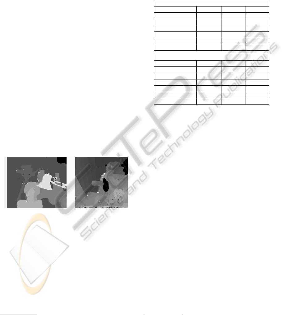
Figure 1: Best (SP)-energy disparity maps for the consid-

ered sequences.

For the Potts model (SP) between 10% and 25%

of all label constellations could be excluded a priori,

and exploiting this knowledge reduces the number of

required iterations for the smooth approximations by

a third. An evaluation of all methods is given in table

1. Here, the augmented Lagrangian (AL) method pro-

vides the tightest lower bounds, the smooth approxi-

mations are signiﬁcantly lower but lead to better inte-

gral solutions. TRW-S is a generally good performing

method. In terms of memory, expansion moves are

lowest (140 MB on Teddy), followed by the convex

http://research.microsoft.com/en-

us/downloads/dad6c31e2c04471fb724ded18bf70fe3/

http://vision.middlebury.edu/stereo/.

Table 1: Stereo: Comparison of lower bounds and integral

energies for (SP) with λ = 15 on the Tsukuba and Teddy

sequences. TRW-S was run for 1500 iterations where it was

near convergence. MPLP (being slower) was run for 500

iterations, where it was progressing only slowly. “Reﬁned”

denotes a subsequent expansion move process. “low. bd.“

reports lower bounds. Note that TRW-S ﬁnds tight lower

bounds much earlier than MPLP.

Tsukuba

method low. bd. integral reﬁned

TRW-S 347222 347274 347234

MPLP 347150 348037 347238

conv (ε = 10

−3

) 346908 347256 347235

conv (ε = 10

−4

) 347193 347251 347236

Lag. 12 × 500 347224 347294 347236

Expansion Move – 347833 347833

Teddy

method low. bd. integral reﬁned

TRW-S 664952 666388 665834

MPLP 664278 669431 665357

conv (ε = 10

−3

) 663073 666472 665153

conv (ε = 10

−4

) 664818 666317 665141

Lag. 12 × 500 664991 666357 665178

Expansion Move – 666631 666631

relaxation (340 MB), TRW-S (560) and our MPLP

(950). With 1.7 GB AL needs too much – all tran-

sitions require explicit storage.

In practice, TRW-S gives comparable integral so-

lutions already after 150 iterations (250 sec.), and al-

ready after 35 it beats the value MPLP ﬁnds after 500

iterations. Hence, TRW-S is clearly superior to MPLP

on this problem.

To save running time it is better to choose a large

ε (e.g. 0.01) for the smooth approximations. Then

500 iterations (2200 sec) sufﬁce, and on the GPU this

should be much faster. Our MPLP implementation

has similar running times, but AL cannot compete

with them.

Motion. For motion it is both common and sensi-

ble to pre-smooth the considered images, so we apply

three iterations of binomial smoothing (but see next

section). We consider two sequences, shown in Fig.

2, where the entire image is moving. For the upper

we take displacements in [−8,8] × [−8,8] in steps of

1, for the lower we take a range of [−5,5] ×[−5,5] in

steps of 0.5. Up to 4% of the labels could be excluded

via Proposition 1.

Table 2 shows that the TRW-S method generally

gives the best results. MPLP gets close, but already

after 95 iterations TRW-S achieves the bound MPLP

ﬁnds after 500. The two methods need nearly equally

long for an iteration

We use edges of type “general” for TRW-S everywhere.

Memory and run-time can be improved (Shekhovtsov et al.,

2008) by changing some of them to type “Potts”.

ICPRAM 2012 - International Conference on Pattern Recognition Applications and Methods

Table 2: Motion: Comparison of lower bounds and integral

energies for (MA) with λ = 1 on the Flower Garden and

Person Walking sequences. TRW-S and MPLP were run for

2500 iterations (close to convergence), with TRW-S using

edges of type “general”. Note that TRW-S ﬁnds tight lower

bounds much earlier than MPLP.

Flower Garden

method low. bd. integral reﬁned

TRW-S 134532 135702 134919

MPLP 134385 137171 134896

conv(ε = 10

−2

) 132463 137212 134993

conv(ε = 10

−3

) 134368 136973 134930

aug-lag 12 × 500 134564 137314 134967

Expansion Move – 136180 136180

Person Walking

method low. bd. integral reﬁned

TRW-S 107358 109014 107937

MPLP 107298 110079 107900

conv(ε = 10

−2

) 105538 117761 108115

conv(ε = 10

−3

) 107268 116821 108128

aug-lag 12 × 500 107069 121581 108931

Expansion Move – 111730 111730

Figure 2: Input sequences (www.cs.brown.edu/ black/) and

ﬂow ﬁelds (color-coded) corresponding to the best (MA)-

energies.

In one case AL gives the best bound, but this

seems to be an exception (see below). The smooth

approximation needs a small ε to give tight bounds.

However, this method and MPLP need the least mem-

ory of all relaxation-based methods (500 MB com-

pared to 3 GB for TRW-S and 1 GB for AL ) and

is furthermore easily implemented in parallel on the

GPU. Again, expansion moves need much less mem-

ory than all relaxation-based methods: 200 MB.

Concerning the optimization of run-times, again

TRW-S wins: it can be terminated after 10 minutes

(on Flower Garden) and still gives a quite tight lower

bound. For the smooth approximations, we found that

with a choice of ε = 0.01 5000 iterations give compa-

rable integral solutions and still useful lower bounds

and runs in 30 min. on a GPU. AL gave useful results

after 6 × 200 iterations, which took roughly 1 hour.

Weak Data Terms. Finally, we consider problems

with more difﬁcult data terms, where we introduce

noise on the stereo images and no longer pre-smooth

those for motion. For stereo, there are very little

changes. For motion we draw three conclusions:

Firstly, AL now breaks down, requiring many more

iterations to produce competitive bounds. Secondly,

TRW-S is now even more superior to MPLP - it needs

50 iterations to produce the same bound as MPLP

after 500. Thirdly, the lower bounds are now much

looser, up to 12% away from the best known integral

solutions. Moreover, the thresholded solutions abso-

lutely need the reﬁnement process.

7 CONCLUSIONS

We have considered several relaxation-based tech-

niques for the problems of motion and stereo with

discretized displacement sets. In summary, the fastest

and most memory saving methods available are not

relaxation-based at all: the expansion moves win.

However, combining them with convex relaxations

gives better results as well as tight lower bounds.

TRW-S is generally the best relaxation-based

strategy to get good solutions very fast, and is

clearly superior to MPLP. Smooth approximations of-

ten need less memory, are parallelizable and work

about equally good. Augmented Lagrangians need

very much memory and, although they give very tight

bounds in some cases, they do not perform good in

general. To facilitate further research in this area, the

source code associated to this paper will be published.

ACKNOWLEDGEMENTS

We thank Fredrik Kahl for helpful discussions. This

work was funded by the European Research Council

(GlobalVision grant no. 209480).

REFERENCES

Bertsekas, D. (1999). Nonlinear Programming, 2nd edition.

Athena Scientiﬁc.

Bhusnurmath, A. and Taylor, C. J. (2008). Solving stereo

matching problems using interior point methods. In

Fourth International Symposium on 3D Data Process-

ing, Visualization and Transmission, 3DPVT.

Boykov, Y., Veksler, O., and Zabih, R. (2001). Fast ap-

proximate energy minimization via graph cuts. IEEE

COMPARING LINEAR AND CONVEX RELAXATIONS FOR STEREO AND MOTION

Transactions on Pattern Analysis and Machine Intel-

ligence (PAMI), 23(11):1222–1239.

Bruhn, A. (2006). Variational optic ﬂow computation: Ac-

curate modelling and efﬁcient numerics. PhD thesis,

Universit

at des Saarlandes, Saarbr

ucken, Germany.

Dantzig, G. and Thapa, M. (1997). Linear Programming 1:

Introduction. Springer Series in Operations Research.

Springer.

Desmet, J., Maeyer, M. D., Hazes, B., and Lasters, I.

(1992). The dead-end elimination theorem and its use

in protein side-chain positioning. Nature, 356:539–

542.

Felzenszwalb, P. and Huttenlocher, D. (2006). Efﬁcient be-

lief propagation for early vision. International Jour-

nal on Computer Vision (IJCV), 70(1).

Globerson, A. and Jaakkola, T. (2007). Fixing max-product:

Convergent message passing algorithms for MAP re-

laxations. In Conference on Neural Information Pro-

cessing Systems (NIPS), Vancouver, Canada.

Glocker, B., Komodakis, N., Tziritas, G., Navab, N., and

Paragios, N. (2008). Dense image registration through

MRFs and efﬁcient linear programming. Medical Im-

age Analysis, 12:731–741.

Goldl

ucke, B. and Cremers, D. (2010). Convex relaxation

for multilabel problems with product label spaces. In

European Conference on Computer Vision (ECCV),

Iraklion, Greece.

Goldstein, T., Bresson, X., and Osher, S. (2009). Global

minimization of Markov random ﬁelds with applica-

tions to optical ﬂow. Technical Report 09-77, UCLA

CAM report.

Horn, B. and Schunck, B. (1981). Determining optical ﬂow.

Artiﬁcial Intelligence, 17:185–203.

Ishikawa, H. (2003). Exact optimization for Markov Ran-

dom Fields with convex priors. IEEE Transactions

on Pattern Analysis and Machine Intelligence (PAMI),

25(10):1333–1336.

Klaus, A., Sormann, M., and Karner, K. (2006). Segment-

based stereo matching using adaptive cost aggregation

and dynamic programming. In International Con-

ference on Pattern Recognition (ICPR), Hong Kong,

China.

Kleinberg, J. and Tardos, E. (1999). Approximation al-

gorithms for classiﬁcation problems with pairwise

relationships: metric labeling and Markov Random

Fields. In Symposium on Foundations of Computer

Science.

Kolmogorov, V. (2006). Convergent tree-reweighted mes-

sage passing for energy minimization. IEEE Trans-

actions on Pattern Analysis and Machine Intelligence

(PAMI), 28(10):1568–1583.

Lellmann, J., Becker, F., and Schn

orr, C. (2009). Con-

vex optimization for multi-class image labeling by

simplex-constrained total variation. In IEEE Interna-

tional Conference on Computer Vision (ICCV), Kyoto,

Japan.

Meltzer, T., Yanover, C., and Weiss, Y. (2005). Globally

optimal solutions for energy minimization in stereo

vision using reweighted belief propagation. In IEEE

International Conference on Computer Vision (ICCV),

Beijing, China.

Memin, E. and Perez, P. (1998). Dense estimation and

object-based segmentation of the optical ﬂow with ro-

bust techniques. IEEE Transactions on Image Pro-

cessing (TIP), 7(5):703–719.

Michelot, C. (1986). A ﬁnite algorithm for ﬁnding the

projection of a point onto the canonical simplex of

. Journal on Optimization Theory and Applica-

tions, 50(1).

Nesterov, Y. (2004). Introductory lectures on convex op-

timization. Applied Optimization. Kluwer Academic

Publishers.

Nesterov, Y. (2005). Smooth minimization of non-smooth

functions. Mathematical Programming, 103(1):127–

152.

Papenberg, N., Bruhn, A., Brox, T., Didas, S., and Weick-

ert, J. (2006). Highly accurate optic ﬂow computa-

tion with theoretically justiﬁed warping. International

Journal on Computer Vision (IJCV), 67(2):141–158.

Pock, T., Schoenemann, T., Cremers, D., and Bischof, H.

(2008). A convex formulation for continuous multi-

label problems. In European Conference on Computer

Vision (ECCV), Marseille, France.

Scharstein, D. and Szeliski, R. (2002). A taxonomy and

evaluation of dense two-frame stereo correspondence

algorithms. International Journal on Computer Vision

(IJCV), 47(1–3):7–42.

Shekhovtsov, A., Kovtun, I., and Hlav

c, V. (2008). Ef-

ﬁcient MRF deformation model for non-rigid image

matching. Computer Vision and Image Understand-

ing, 112(1):91–99.

Sontag, D., Globerson, A., and Jaakkola, T. (2010). Intro-

duction to dual decomposition for inference. In Opti-

mization for Machine Learning. MIT Press.

Szeliski, R., Zabih, R., Scharstein, D., Veksler, O., Kol-

mogorov, V., Agarwala, A., Tappen, M., and Rother,

C. (2008). A comparative study of energy min-

imization methods for Markov random ﬁelds with

smoothness-based priors. IEEE Transactions on

Pattern Analysis and Machine Intelligence (PAMI),

30(6):1068–1080.

Trobin, W., Pock, T., Cremers, D., and Bischof, H. (2008).

An unbiased second-order prior for high-accuracy

motion estimation. In Pattern Recognition (Proc.

DAGM), Munich, Germany.

Wainwright, M., Jaakkola, T., and Willsky, A. (2005). MAP

estimation via agreement on (hyper-)trees: Message-

passing and linear programming approaches. IEEE

Tansactions on Information Theory, 51(11):3697–

3717.

Woodford, O., Torr, P., Reid, I., and Fitzgibbon, A.

(2008). Global stereo reconstruction under second

order smoothness priors. In IEEE Computer Society

Conference on Computer Vision and Pattern Recogni-

tion (CVPR), Anchorage, Alaska.

Yang, Q., Wang, L., Yang, R., Stew

enius, H., and Nist

er,

D. (2009). Stereo matching with color-weighted cor-

relation, hierarchical belief propagation and occlusion

handling. IEEE Transactions on Pattern Analysis and

Machine Intelligence (PAMI), 31(3):492–504.

Zach, C., Gallup, D., Frahm, J.-M., and Niethammer, M.

(2008). Fast global labeling for real-time stereo us-

ing multiple plane sweeps. In Vision, Modeling and

Visualization Workshop (VMV), Konstanz, Germany.

Zach, C., Pock, T., and Bischof, H. (2007). A duality based

approach for realtime TV-L1 optical ﬂow. In Pattern

Recognition (Proc. DAGM), Heidelberg, Germany.

ICPRAM 2012 - International Conference on Pattern Recognition Applications and Methods