
WHY COLOR CONSTANCY IMPROVES FOR MOVING OBJECTS
Marc Ebner
Ernst-Moritz-Arndt-Universit
¨
at Greifswald, Institut f
¨
ur Mathematik und Informatik
Walther-Rathenau-Straße 47, 17487 Greifswald, Germany
Keywords:
Color constancy, Color perception, Computational modeling, Object/scene motion.
Abstract:
Light which is measured by retinal receptors varies with the illuminant. However, a human observer is able
to discount the illuminant and to accurately determine the color of objects. The human brain computes a
color constant descriptor which is approximately independent of the illuminant. This ability is called color
constancy. Recently, it has been shown that color constancy improves for a moving stimulus. It has been
argued that high level motion areas may have an influence on the computation of a color constant descriptor.
We have developed a computational model for color perception which can be mapped to the different stages of
the human visual system. We test our model with two types of stimuli: stationary and moving. In our model,
color constancy is computed purely bottom up. Our model also shows better color constancy for a moving
stimulus. This indicates that an influence from high level motion areas is not required.
1 MOTIVATION
A human observer is able to perceive the color of ob-
jects as approximately color constant. This ability is
know as Color Constancy (Zeki, 1993; Ebner, 2007a).
Consider a scene with one or more light sources. The
light is illuminating the objects of the scene. Some of
the light is absorbed while the remaining light is re-
flected by the objects. Eventually, the light enters the
eye where it is measured by the retinal receptors. The
brain is able to compute a color constant descriptor
from the light entering the eye even though this light
varies with the color of the illuminant.
Suppose that an illuminant with a lot of energy in
the red and green parts of the spectrum illuminates the
scene. For such an illuminant, a digital sensor (with
neutral white balance) will measure an image with a
yellowish color cast. If the illuminant emits its light
primarily in the blue part of the spectrum, then the
digital image will have a bluish color cast. The prob-
lem of computing a color constant descriptor based
only on data measured by the retinal receptors is actu-
ally underdetermined. Nevertheless, the brain some-
how does arrive at a color constant descriptor which is
independent of the illuminant. Cells found in V4 re-
spond in a color constant way (Zeki and Marini, 1998;
Zeki and Bartels, 1999). For instance, certain cells re-
spond whenever a yellowish object enters the recep-
tive field of this cell irrespective of the light which is
actually reflected from the object.
Quite a number of computational algorithms have
been proposed which address the problem of color
constancy. (Land, 1974) has proposed the Retinex
theory and together with McCann developed the first
computational algorithm for color constancy (Land
and McCann, 1971). The Retinex algorithm consid-
ers random paths running along an image created by
a matrix of receptors with a logarithmic response. A
color constant descriptor is computed by subtracting
the data measured by adjacent receptors, applying a
threshold function and then summing up the result.
Extensions to the original Retinex algorithm have
been proposed by (Horn, 1974) and (Blake, 1985).
(Moore et al., 1991) have implemented a version of
the Retinex algorithm in hardware. (Funt et al., 2004)
give an implementation in Matlab.
Apart from the Retinex algorithm, several other
algorithms have been proposed, e.g. the gray-world-
assumption (Buchsbaum, 1980), recovery of basis-
functions (Maloney and Wandell, 1986) or gamut-
constraint methods (Forsyth, 1990). Most color con-
stancy algorithms assume that the scene is uniformly
illuminated. However, in practice multiple illumi-
nants are present which cause a non-uniform illumi-
nation. For instance, some daylight may be falling
through a window while an artificial illuminant may
be switched on inside the room. Land and McCann’s
Retinex algorithm (Land and McCann, 1971) also
works in the presence of a non-uniform illuminant.
(Barnard et al., 1997) has extended the gamut con-
193
Ebner M..
WHY COLOR CONSTANCY IMPROVES FOR MOVING OBJECTS.
DOI: 10.5220/0003711301930198
In Proceedings of the International Conference on Bio-inspired Systems and Signal Processing (BIOSIGNALS-2012), pages 193-198
ISBN: 978-989-8425-89-8
Copyright
c
2012 SCITEPRESS (Science and Technology Publications, Lda.)

straint algorithm to scenes with non-uniform illumi-
nation. Neural architectures for color constancy have
also been proposed (D’Zmura and Lennie, 1986; Du-
fort and Lumsden, 1991). As of now, it is not clear
which algorithm is used by the brain to arrive at a
color constant descriptor. Most computational algo-
rithms for color constancy are quite complex and can-
not readily be mapped to what is known about the hu-
man visual system. (Ebner, 2007b) has established a
correspondence between his algorithm which is based
on the computation of local space average color and
the workings of the human visual system.
In a recent study, (Werner, 2007) has shown that,
when an object moves, color constancy improves.
Werner argues that high-level motion processing (at-
tention driven) has an impact on color perception.
With this contribution, we 1) extend Ebner’s (2007a)
color constancy model for color perception and 2) use
this model to show how color constancy can improve
if an object moves. This supports the hypothesis that
Werner’s results may be explained purely bottom up
without the direct influence from high-level vision ar-
eas to color processing areas.
2 COLOR IMAGE FORMATION
In order to understand the computational model for
color perception which is detailed in the next sec-
tion, we first need a model of color image formation.
Three types of cones can be distinguished (Dartnall
et al., 1983). The retinal receptors respond to light in
the red, green and blue parts of the spectrum (cones).
We will use (x, y) coordinates to index the retinal re-
ceptors. The non-uniform spatial distribution of the
receptors is of no concern in this context. Each re-
ceptor located at position (x,y) receives light from a
corresponding object patch of the scene. Let L(x,y,λ)
be the irradiance falling onto the corresponding ob-
ject patch for wavelength λ. Some of the irradiance
is absorbed while the remainder is reflected into the
surrounding. We assume that the objects are mainly
diffuse reflectors, i.e. the incident light is reflected
uniformly into the surrounding. The dichromatic re-
flectance model could be taken into account to model
highlight reflections. However, they are usually lo-
calized and hence have a small impact on the model
described here.
Let R(x,y,λ) be the percentage of the reflected
light at corresponding object position (x,y) and wave-
length λ. Let S
i
(λ) be the sensitivity of cone i ∈
{r,g,b} for wavelength λ. Then the energy I
i
(x,y)
measured by retinal receptor i at position (x,y) can be
modeled as (Ebner, 2007a)
I
i
(,x, y) = G(x,y)
Z
S
i
(λ)R(x,y,λ)L(x, y, λ)dλ. (1)
where G(x,y) = cos(α(x, y)) is a geometry factor
which depends on the scene geometry, i.e. the an-
gle α between the normal vector and the direction to
the light source at position (x, y). In case of an ideal
receptor which responds only to a single wavelength
λ
i
, i.e. with S
i
(λ) = δ(λ − λ
i
), we obtain
I
i
(,x, y) = G(x,y)R(x, y,λ
i
)L(x,y,λ
i
). (2)
Thus, we see that the measured light at retinal posi-
tion (x,y) is proportional to the reflectance R and the
irradiance L. Let I(x,y) = [I
r
(x,y), I
g
(x,y), I
b
(x,y)] be
the measured light at retinal position, and R(x,y) =
[R(x,y,λ
r
),R(x, y,λ
g
),R(x, y,λ
b
)] be the reflectance
and L(x,y) = [L(x, y, λ
r
),L(x, y, λ
g
),L(x, y, λ
b
)] be the
irradiance at the corresponding object point, then we
write
I(x,y) ∝ R(x,y) · L(x, y) (3)
where · denotes component-wise multiplication. It is
of course clear, that the retinal receptors are not nar-
row band. However, considering them as narrow band
will allow us better to understand how the brain ar-
rives at a color constant descriptor. Not having narrow
band receptors complicates the performance of color
constancy. Human color constancy correlates with re-
flectance estimation but is not perfect (McCann et al.,
1976).
3 COMPUTATIONAL MODELING
OF COLOR PERCEPTION
(Ebner, 2007b) has given a computational model of
color constancy which estimates reflectance. It is
based on the computation of local space average color
(Ebner, 2009). Here, we provide an extended ver-
sion of this model. The retinal receptors respond
to the incoming light. Three types of receptors are
modeled which absorb the light in the red, green and
blue parts of the spectrum as described above. Let c
be the energy measured by the receptors. All chan-
nels are scaled by the maximum value m with m =
max
i,x,y
I
i
(x,y). This models the adaptation mecha-
nism of the eye. We obtain
c(x,y) =
I(x,y)
m
(4)
for the measured light c which also takes adaptation
into account. The retinal cells also capture light from
different directions as the eye or the stimulus moves.
Let
˜
c be the output of this temporal averaging, i.e.
˜
c(x,y) = (1 − p
t1
)
˜
c(x,y) + p
t1
c(x,y) (5)
BIOSIGNALS 2012 - International Conference on Bio-inspired Systems and Signal Processing
194

with p
t1
= 0.8.
The response of the retinal receptors can be mod-
eled using either a logarithmic response curve as sug-
gested by (Faugeras, 1979) or using a square root
or cube root response curve as suggested by (Hunt,
1957). We will assume a cube root response func-
tion. The cube root response is also used for the CIE
L
∗
u
∗
v
∗
color space (International Commission on Il-
lumination, 1996). All these different types of re-
sponse curves can be used to approximate each other
on a given range and with the right parameters (Ebner
et al., 2007). Hence, the output of the retinal receptors
o
r
is given by
o
r
=
˜
c
1/3
. (6)
The three retinal receptors create a three dimen-
sional color space. Each measurement is represented
by a point in this coordinate space. The color oppo-
nent and double opponent cells of V1 (Livingstone
and Hubel, 1984; Tov
´
ee, 1996) transform this RGB
color space to a rotated color space where the axes
are dark-bright, red-green and blue-yellow. We do
not incorporate this rotation of the color space into
our computational model because the outcome is the
same irrespective of the orientation of the coordinate
system. Hence, we will omit this rotation here. Thus,
we obtain for the signal processed in V1, o
V1
= o
r
.
Cells found in V4 have been shown to respond in
a color constant way (Zeki and Marini, 1998). Hence,
we assume that the essential processing, which is re-
quired to compute a color constant descriptor, is lo-
cated in V4. In our model, gap junctions between neu-
rons in V4 create a resistive grid. Gap junctions are
known to behave like resistors (Herault, 1996). The
resistive grid is used to compute local space average
color. Because of the resistive connection between
adjacent neurons, some of the activation is exchanged
between connected neurons. Let N(x,y) be the set of
neighboring neurons which are connected to a given
neuron which processes information from retinal po-
sition (x, y). Thus, each neuron of the resistive grid
computes local space average color a(x, y) iteratively
using the update equations
a
0
(x,y) :=
1
|N(x,y)|
∑
(x
0
,y
0
)∈N(x,y)
a(x
0
,y
0
) (7)
a(x,y) := o
r
(x,y) · p
a
+ a
0
(x,y) · (1 − p
a
). (8)
First, local space average color from neighboring neu-
rons is averaged. The second step adds a little amount
from the retinal input o
r
to the average which has been
computed so far using a weighted average with the pa-
rameter p
a
. The smaller the parameter p
a
the larger
the support over which local space average color is
computed. For p
a
→ 0, global space average color
is computed. This is illustrated in Figure 1 where
local space average color is computed using differ-
ent values of p
a
. For our experiment, we have used
p
a
= 0.000758. This value is chosen such that local
space average color is computed over a sufficiently
large area, e.g. 30% of the image. A color constant
descriptor is computed in the next stage. Because this
requires additional neural circuitry, the signal is again
temporally averaged. Let
˜
a be the temporal average
of local space average color, then
˜
a is computed using
˜
a(x,y) := p
t2
a(x,y) + (1 − p
t2
)
˜
a(x,y) (9)
with p
t2
= 0.1.
In Ebner’s (2007a) model, local space average
color a is subtracted from the measured color o
r
to
arrive at a color constant descriptor. Thus, we com-
pute
o
V4
(x,y) := o
V1
(x,y) −
˜
a(x,y). (10)
The components of our model for color perception are
illustrated in Figure 2. The color constant descriptor
o
V4
has to be transformed before its data can be visu-
alized using an RGB color space. In order to evaluate
the performance of our computational model, we ba-
sically invert the pipeline as described above. In the
coordinate space of the color constant descriptor, gray
lies at the center of this space. First we have to apply
a shift of the coordinate system followed by the in-
verse of the cube root function to obtain a reflectance
estimate. The necessary shift can be computed by as-
suming a uniform distribution of colors. In this case,
the shift is given as d = [k, k, k] with
k =
n
∑
i=0
i
n
1
3
. (11)
The estimated reflectance
˜
R is then given as
˜
R = (|o
V4
+ d|)
3
. (12)
4 COMPUTATION OF A COLOR
CONSTANT DESCRIPTOR
The color constant descriptor is computed by sub-
tracting local space average color a from the mea-
sured color o
V1
(Ebner, 2007b). Local space aver-
age color computed by a resistive grid can be approx-
imated by the following function (Ebner, 2009)
a(x,y) = k(x,y)
Z Z
x
0
,y
0
g(x − x
0
,y − y
0
)o
V1
dx
0
dy
0
(13)
where g(x,y) is a smoothing kernel and k(x,y) is a
scaling factor with
k(x, y) =
1
R R
x
0
,y
0
g(x − x
0
,y − y
0
)dx
0
dy
0
. (14)
WHY COLOR CONSTANCY IMPROVES FOR MOVING OBJECTS
195
(a) (b) (c) (d)
Figure 1: (a) input image (size 614 × 410) (b-d) spatially averaged images (b) p
a
= 0.005 (c) p
a
= 0.0002 (d) p
a
= 0.00001.
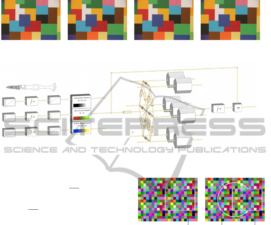
V1
Retinal Receptor
V4
Figure 2: Computational model for color perception.
The smoothing kernel g(x,y) can be approximated by
the following function with smoothing parameter σ.
g(x,y) = e
−
|x|+|y|
σ
(15)
The smoothing parameter depends on the parameter
p
a
with σ =
1−p
a
4p
a
. As we have described above, the
response of the retinal receptors can be described by a
cube root function or by a logarithmic function. Both
functions are similar with a proper choice of parame-
ters on the relevant data range. Using o
V1
∝ log(RL),
we obtain a color constant descriptor o
V1
− a(x, y) =
logR(x, y)−constant. Note that in order to obtain this
result, we have used the assumption that the illumi-
nant varies slowly with respect to the support of the
smoothing kernel, i.e. L(x,y) can be considered con-
stant within the support. Similarly, it is assumed that
several different reflectances are contained with in the
area of support of the smoothing kernel.
5 EXPERIMENTS
Two types of stimuli are used in order to investigate
the impact of motion on color constancy: A) station-
ary stimulus and B) moving stimulus. For stimulus
A a stationary test patch is viewed in front of a sta-
tionary background. For stimulus B the same test
patch moves across the background. The observer is
assumed to fixate the test patch. These two stimuli
Stimulus B
moving
crop regioncircular motioncrop region
Stimulus A
stationary
Figure 3: The stationary stimulus (A) is created by cropping
a rectangular area from a larger random color checkerboard
pattern. The moving stimulus (B) is created by moving the
crop region along a circular path.
are evaluated with respect to the ability to compute a
color constant descriptor.
The two stimuli originate from a random color
checkerboard pattern as shown in Figure 3. For stim-
ulus A, a smaller rectangular area is cropped from a
larger checkerboard pattern. The test patch is overlaid
in the center. The pattern stays stationary throughout
the experiment. For stimulus B, the crop area moves
in a circular motion across the background. Again,
the test patch is displayed in the center of the crop
area. All of the colors which have been used to gen-
erate the stimuli have been chosen at random.
Figure 4 shows the results for the two stimuli after
4320 iterations of the algorithm described in Section
3. The resistive grid of V4 is used to compute local
space average color which is an estimate of the illu-
BIOSIGNALS 2012 - International Conference on Bio-inspired Systems and Signal Processing
196
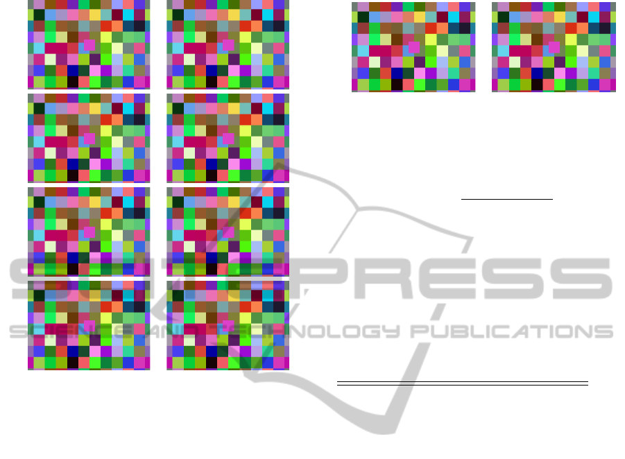
Stimulus A Stimulus B
ReflectanceR
Receptor o
r
LSA Color
˜
a
Estimated R.
˜
R
Figure 4: The first column shows the results when a static
input stimulus is used. The second column shows the re-
sults when a moving stimulus is used. The first row of
images shows the reflectance images R. The second row
shows the input stimulus c. The third row shows the es-
timate of the illuminant, i.e. local space average color
˜
a.
The fourth row shows the internal color constant descriptor
transformed back into RGB values
˜
R. It is clear that the
estimate of the illuminant improves greatly when the input
stimulus moves.
minant. It is clear that for stimulus B, local space
average color
˜
a provides a much better estimate of
the illuminant. This is because the background moves
relative to the retinal receptors. Hence, local space
average color is much smoother than for stimulus A.
For a static stimulus, the retinal receptors are always
exposed to the same input. Therefore, local space av-
erage color computed within one of the color patches
is slightly biased towards the color of the patch. Fig-
ure 5 illustrates this bias for both stimuli. The bias
image is computed by transforming local space aver-
age color back to RGB space and then dividing by the
color of the illuminant.
We have repeated this experiment for 100 random
starting positions of the crop region and also for 10
randomly chosen illuminants. In total 1000 experi-
ments were performed. In order to evaluate the abil-
ity to compute a color constant descriptor, we com-
pute the angular error e(x, y) between the estimated
reflectance
˜
R(x,y) and the actual reflectance R(x,y).
Stimulus A Stimulus B
Bias
Figure 5: Bias due to the input stimulus. For stimulus A the
bias is more pronounced. For stimulus B the estimate of lo-
cal space average color is much better, hence the reflectance
estimate is more accurate compared to stimulus A.
e(x,y) = cos
−1
˜
R(x,y)R(x, y)
|
˜
R(x,y)||R(x, y)|
(16)
Table 1 shows the average angular error ¯e (aver-
age angular error over all image pixels and over all
1000 experiments) for the two stimuli A and B. The
standard deviation is also shown. The angular error is
significantly lower (t-test t = 182.7) when the back-
ground moves behind the test patch.
Table 1: Average angular error ¯e across all image pixels and
all 1000 experiments.
Angular Error ¯e Std. Dev.
Stimulus A 6.0120 0.1507
Stimulus B 2.8283 0.1012
(Werner, 2007) has shown that motion improves
the ability to correctly estimate the color of a given
test patch. Werner argued that high-level motion pro-
cessing may influence the computation of a color con-
stant descriptor and that color processing and motion
processing may not be completely separated. Here,
we have given a computational model of color percep-
tion which shows the same behavior, i.e. color can be
estimated better if the retinal receptors move across a
background. In our model, color is computed bottom
up. No high-level motion areas are simulated.
According to our view, motion processing does
not have a direct impact on the computation of a color
constant descriptor. Instead, motion processing is
used to control the motion of the eye ball. If a test
patch moves across a stationary background and the
eye fixates the test patch, then the background moves
behind the test patch in the same way that the back-
ground moved behind the test patch in our experi-
ments. This causes the retinal receptors to be exposed
to different inputs in the course of time. Because of
the temporal integration, a more accurate estimate of
the illuminant is obtained.
WHY COLOR CONSTANCY IMPROVES FOR MOVING OBJECTS
197

6 CONCLUSIONS
We have given a computational model for color per-
ception. The retinal response is assumed to follow a
cube root relationship. The first stage is adaptation
followed by a temporal averaging process. By the
time the visual stimulus has reached V1, a rotation
of the coordinate system has occurred. In V4, local
space average is computed through a resistive grid.
This resistive grid is created by neurons which are lat-
erally connected via gap-junctions. A color constant
descriptor is computed by subtracting local space av-
erage color from the signal which is received from
V1. Another temporal averaging occurs at the last
stage. We have shown that this model is able to re-
produce an important result from experimental psy-
chology, namely that color constancy improves for a
moving stimulus.
REFERENCES
Barnard, K., Finlayson, G., and Funt, B. (1997). Color con-
stancy for scenes with varying illumination. Computer
Vision and Image Understanding, 65(2):311–321.
Blake, A. (1985). Boundary conditions for lightness com-
putation in mondrian world. Computer Vision, Graph-
ics, and Image Processing, 32:314–327.
Buchsbaum, G. (1980). A spatial processor model for object
colour perception. Journal of the Franklin Institute,
310(1):337–350.
Dartnall, H. J. A., Bowmaker, J. K., and Mollon, J. D.
(1983). Human visual pigments: microspectrophoto-
metric results from the eyes of seven persons. Proc.
R. Soc. Lond. B, 220:115–130.
Dufort, P. A. and Lumsden, C. J. (1991). Color categoriza-
tion and color constancy in a neural network model of
V4. Biological Cybernetics, 65:293–303.
D’Zmura, M. and Lennie, P. (1986). Mechanisms of color
constancy. Journal of the Optical Society of America
A, 3(10):1662–1672.
Ebner, M. (2007a). Color Constancy. John Wiley & Sons,
England.
Ebner, M. (2007b). How does the brain arrive at a color con-
stant descriptor? In Mele, F., Ramella, G., Santillo, S.,
and Ventriglia, F., eds., Proc. of the 2nd Int. Symp. on
Brain, Vision and Artificial Intelligence, Naples, Italy,
pp. 84–93, Berlin. Springer.
Ebner, M. (2009). Color constancy based on local space av-
erage color. Machine Vision and Applications Journal,
20(5):283–301.
Ebner, M., Tischler, G., and Albert, J. (2007). Integrating
color constancy into JPEG2000. IEEE Transactions
on Image Processing, 16(11):2697–2706.
Faugeras, O. D. (1979). Digital color image processing
within the framework of a human visual model. IEEE
Trans. on, ASSP-27(4):380–393.
Forsyth, D. A. (1990). A novel algorithm for color con-
stancy. Int. J. of Computer Vision, 5(1):5–36.
Funt, B., Ciurea, F., and McCann, J. (2004). Retinex in
MATLAB. Journal of Electronic Imaging, 13(1):48–
57.
Herault, J. (1996). A model of colour processing in the
retina of vertebrates: From photoreceptors to colour
opposition and colour constancy phenomena. Neuro-
computing, 12:113–129.
Horn, B. K. P. (1974). Determining lightness from an im-
age. Comp. Graphics and Image Processing, 3:277–
299.
Hunt, R. W. G. (1957). Light energy and brightness sensa-
tion. Nature, 179:1026–1027.
International Commission on Illumination (1996). Col-
orimetry, 2nd ed., Tech. Report 15.2.
Land, E. H. (1974). The retinex theory of colour vision.
Proc. Royal Inst. Great Britain, 47:23–58.
Land, E. H. and McCann, J. J. (1971). Lightness and retinex
theory. J. of the Optical Society of America, 61(1):1–
11.
Livingstone, M. S. and Hubel, D. H. (1984). Anatomy and
physiology of a color system in the primate visual cor-
tex. The Journal of Neuroscience, 4(1):309–356.
Maloney, L. T. and Wandell, B. A. (1986). Color constancy:
a method for recovering surface spectral reflectance. J.
of the Optical Society of America A, 3(1):29–33.
McCann, J. J., McKee, S. P., and Taylor, T. H. (1976).
Quantitative studies in retinex theory. Vision Res.,
16:445–458.
Moore, A., Allman, J., and Goodman, R. M. (1991). A real-
time neural system for color constancy. IEEE Trans-
actions on Neural Networks, 2(2):237–247.
Tov
´
ee, M. J. (1996). An introduction to the visual system.
Cambridge University Press, Cambridge.
Werner, A. (2007). Color constancy improves, when an ob-
ject moves: High-level motion influences color per-
ception. Journal of Vision, 7(14):1–14.
Zeki, S. (1993). A Vision of the Brain. Blackwell Science,
Oxford.
Zeki, S. and Bartels, A. (1999). The clinical and func-
tional measurement of cortical (in)activity in the vi-
sual brain, with special reference to the two subdivi-
sions (V4 and V4α) of the human colour centre. Proc.
R. Soc. Lond. B, 354:1371–1382.
Zeki, S. and Marini, L. (1998). Three cortical stages
of colour processing in the human brain. Brain,
121:1669–1685.
BIOSIGNALS 2012 - International Conference on Bio-inspired Systems and Signal Processing
198
