
HANDLING IMPRECISE LABELS IN FEATURE SELECTION
WITH GRAPH LAPLACIAN
Gauthier Doquire and Michel Verleysen
Machine Learning Group - ICTEAM, Universit
´
e catholique de Louvain
Place du Levant 3, 1348 Louvain-la-Neuve, Belgium
Keywords:
Feature selection, Imprecise labels, Graph laplacian.
Abstract:
Feature selection is a preprocessing step of great importance for a lot of pattern recognition and machine learn-
ing applications, including classification. Even if feature selection has been extensively studied for classical
problems, very little work has been done to take into account a possible imprecision or uncertainty in the
assignment of the class labels. However, such a situation can be encountered frequently in practice, especially
when the labels are given by a human expert having some doubts on the exact class value. In this paper, the
problem where each possible class for a given sample is associated with a probability is considered. A fea-
ture selection criterion based on the theory of graph Laplacian is proposed and its interest is experimentally
demonstrated when compared with basic approaches to handle such imprecise labels.
1 INTRODUCTION
The feature selection step is known to be of funda-
mental importance for classification problems. Its ob-
jective is to get rid of irrelevant and/or redundant fea-
tures and to identify those being really useful for the
problem. The benefits of feature selection for classifi-
cation can be numerous and include: better prediction
performances of the classification models, easier in-
terpretation of these models, deeper understanding of
the problems and/or reduced feature acquisition and
storage cost (Guyon and Elisseeff, 2003).
Due to its importance, feature selection has been
extensively studied in the literature, especially for
standard classification problems, i.e. for problems
where each sample point is associated without am-
biguity to exactly one class label (see e.g. (Dash and
Liu, 1997; Kwak and Choi, 2002)). It has revealed
extremely useful in many fields among which one can
cite for example text classification (Yang and Ped-
ersen, 1997) or gene expression based classification
(Ding and Peng, 2003).
Quite surprisingly, to the best of our knowledge,
very few attempts have been made up to now to
achieve feature selection in problems where the class
labels are uncertainly or imprecisely specified and can
even be erroneous. However, such a situation can be
frequently encountered in practice and thus deserves
to be investigated. Indeed, it is frequent that a hu-
man supervision is required to assign labels to sample
points. This is for example the case in the medical
domain where a diagnostic has to be made based on
a micro-array or a radiography. Such a task can be
hard to perform and experts sometimes hesitate be-
tween different classes or propose a single class label
but associate it with a measure of the confidence they
have in this label.
In this work, we address the problem of feature
selection in the case where an expert gives, for each
sample x
i
(i = 1 . . . n), a probability value p
i j
to each
possible class c
j
( j = 1 . . . l) such that
∑
l
j=1
p
i j
= 1 ∀i.
Such a supervision has been called possibilistic labels
in the literature; it can also be obtained by combin-
ing the opinion of several experts about the member-
ship of a point to a given class. As a concrete prob-
lem, (Denoeux and Zouhal, 2001) evokes the recog-
nition of certain transient phenomena in EEG data,
whose shapes can be very hard to distinguish from
EEG background activity, even for trained physicians;
experts can rarely be sure about the presence of such
phenomena, but can be able, however, to express a
possibility about this presence. Such labels are also
encountered in fuzzy classification problems. Indeed
when classes are not well defined, they can sometimes
be better represented by fuzzy labels, measuring the
degree of membership of the samples to each of the
classes. This is for example the case when the labels
are obtained through the fuzzy c-means clustering al-
162
Doquire G. and Verleysen M. (2012).
HANDLING IMPRECISE LABELS IN FEATURE SELECTION WITH GRAPH LAPLACIAN.
In Proceedings of the 1st International Conference on Pattern Recognition Applications and Methods, pages 162-169
DOI: 10.5220/0003712101620169
Copyright
c
SciTePress

gorithm (Bezdez and Pal, 1992).
The proposed feature selection algorithm is a
ranking technique based on the Laplacian Score (He
et al., 2006), originally introduced for feature selec-
tion in unsupervised problems. The basic idea is to
select features according to their locality preserving
power, i.e. according to how well they respect a prox-
imity measure defined between samples in an arbi-
trary way. In this paper, it is shown how this criterion
can be extended to the uncertain label framework.
The rest of the paper is organized as follows.
In Section 2, related work on feature selection and
uncertain label analysis is presented. The original
Laplacian Score is described in Section 3 and the pro-
posed new criterion, called weighted Laplacian Score
(WLS), is introduced in Section 4. Section 5 presents
experimental results assessing the interest of WLS be-
fore Section 6 concludes the work.
2 RELATED WORK
As explained above, feature selection has been widely
investigated in the literature; traditional approaches
include wrapper or filter strategies. Wrappers make
use of the prediction (classification or regression)
model to select features in order to maximize the per-
formances of this model. Such methods thus require
building a huge number of prediction models (with
potential hyperparameters to tune) and are typically
slow. However, the performances of the prediction
models with the selected features are expected to be
high (Kohavi and John, 1997).
On the other hand, filters are independent of any
prediction model; they are rather based on a relevance
criterion. The most popular of those criteria include
the correlation coefficient (Hall, 1999), the mutual in-
formation (Peng et al., 2005) and other information-
theoretic quantities (Meyer et al., 2008) among many
more. Filters are in practice faster and much more
general than wrappers since they can be used prior
to any prediction model; they are considered in this
work. More recently, embedded methods, performing
simultaneously feature selection and prediction have
also raised a huge interest (Yuan and Lin, 2006) since
the publication of the original LASSO paper (Tibshi-
rani, 1996).
Classifiers for problems with uncertain label have
also been proposed in the literature; more specifically
the Dempster-Shafer theory of belief functions has
proven to be very successfull in this context (Denoeux
and Zouhal, 2001; Jenhani et al., 2008; C
ˆ
ome et al.,
2009). Indeed, it offers a convenient and very gen-
eral way to model one’s belief about the class label
of a sample. This belief can be expressed as in this
paper but can also take more general forms as a set
of possible class labels or the probability of a class
with no additional information. Moreover, the Trans-
ferable Belief Model (Smets et al., 1991) permits to
combine elegantly the different pieces of belief con-
cerning a sample class membership.
Despite its importance, the problem of feature se-
lection with imprecise class labels has received few
attention in the literature. In (Semani et al., 2004),
the authors consider a fully supervised classification
problem before relabelling automatically all the data
points in order to take into account the classifica-
tion ambiguity. In (Wang et al., 2009), the Hilbert-
Schmidt independence criterion is used to achieve
feature selection with uncertain labels. However, the
possibility of label noise is not studied in this paper
which is rather focused on multi-label like problems.
It is worth noting that more specific weakly super-
vised problems have already been considered in the
literature. This is the case for semi-supervised prob-
lems in which a small fraction of the samples are as-
sociated with an exact class label while no label at all
is associated with the other samples (Chapelle et al.,
2006). An extension of the Laplacian Score has been
proposed for feature selection in this context (Zhao
et al., 2008) while many other methods also exist in
the literature, e.g. (Zhao and Liu, 2007).
A closely related but different problem is the one
where only pairwise constraints between samples are
given. This means that the exact class labels are un-
available but that, for some couples of points, it is
known whether or not they belong to the same class.
Here again, feature selection for this paradigm has
been achieved successfully with an extension of the
Laplacian Score (Zhang et al., 2008).
3 THE LAPLACIAN SCORE
This section briefly presents the Laplacian Score, in-
troduced in (He et al., 2006) for unsupervised fea-
ture selection. As already discussed, the method aims
at selecting the features preserving at most the local
structure of the data, or, in other words, the neigh-
borood relationships between samples.
Let X be a given data set containing m samples x
i
(i = 1 . . . m) and f features f
r
(r = 1 . . . f ). Denote by
f
ri
the r
th
feature of the i
th
sample of X. It is possi-
ble to build a proximity graph representing the local
structure of X. This graph consists in m nodes, each
representing a sample of X. An edge is present be-
tween node i and node j if the corresponding points
x
i
and x
j
in X are close, i.e. if x
i
is among the k nearest
HANDLING IMPRECISE LABELS IN FEATURE SELECTION WITH GRAPH LAPLACIAN
163

neighbors of x
j
or conversely, where k is a parameter
of the method. Traditionally, the proximity measure
used to determine the nearest neighbors of a point is
the Euclidean distance, denoted as d(., .).
Based on this proximity graph, a matrix S can be
built in the following way:
S
i, j
=
(
e
−
d(x
i
,x
j
)
t
if x
i
and x
j
are close
0 otherwise
(1)
with t being a suitable positive constant. We also de-
fine D = diag(S1), with 1 = [1 . . . 1]
T
, as well as the
graph Laplacian L = D − S (Chung, 1997).
The mean of each feature f
r
(weighted by the local
density of the data points) is then removed; the new
features are defined by
˜
f
r
= f
r
−
f
T
r
D1
1
T
D1
1.
The objective of this normalisation is to prevent a
non-zero constant vector such as 1 to be assigned a
zero Laplacian score (and thus to be considered as
highly relevant) as such a feature obviously does not
contain any information. It is then possible to com-
pute the Laplacian score of each feature f
r
as
L
r
=
˜
f
r
T
L
˜
f
r
˜
f
r
T
D
˜
f
r
(2)
and features are ranked according to this score, in in-
creasing order.
More details can be found in the original paper
(He et al., 2006), where the authors also derive a con-
nection between (2) and the canonical Fisher score.
4 THE WEIGHTED LAPLACIAN
SCORE FOR POSSIBILISTIC
LABELS
In this section, the proposed feature selection crite-
rion for possibilistic labels is introduced. As already
stated, all the developments presented here could as
well be applied to the case where an expert only pro-
vides one class label for each point of the training set,
but associates this label with a coefficient indicating
the certainty he has on his prediction. The section
ends with a theoretical justification of the WLS.
4.1 The Proposed Algorithm
Consider again the data set X ∈ ℜ
m× f
. Each sam-
ple point x
i
has a single true class label c
j
belonging
to the set of the l possible class labels c
1
. . . c
l
. In
practice, however, this label is not precisely known.
Instead, each point x
i
is rather associated with a prob-
ability value p
i j
for each possible class label such that
∑
l
j=1
p
i j
= 1 ∀i. These values can be directly obtained
from an expert or come from the combination of sev-
eral experts opinions. Obviously, the probability that
two points in X have the same class label can be com-
puted as follows:
S
sim
i j
=
l
∑
k=1
p
i,k
p
j,k
. (3)
Thus, S
sim
i, j
is simply the scalar product between the
vectors of the labels probability for x
i
and x
j
.
The algorithm starts by building a graph G
sim
with
m nodes, each corresponding to a point in X. An edge
exists between node i and node j if the probability that
the two samples x
i
and x
j
have the same class label is
greater than 0.
From the matrix S
sim
, it is possible to define
D
sim
= diag(S
sim
1) and the graph Laplacian of G
sim
,
L
sim
= D
sim
− S
sim
.
Let us then construct a matrix S
dis
∈ ℜ
m×m
, corre-
sponding to the probabilities that two samples belong
to different classes:
S
dis
i j
= 1 −
c
∑
k=1
p
i,k
p
j,k
= 1 − S
sim
i j
(4)
and let us define D
dis
= diag(S
dis
1) as well as L
dis
=
D
dis
− S
dis
.
The importance of each feature f
r
is eventually
computed by the weighted Laplacian score that we
define to be
W LS
r
=
f
T
r
L
sim
f
r
f
T
r
L
dis
f
r
; (5)
the features can be ranked according to this score, in
increasing order. The number of features to keep to
build the model has to be determined in advance.
4.2 Justification
In the above developements, the graph G
sim
defines a
structure between the points by connecting those pos-
sibly sharing the same clas label. Based on this struc-
ture, the matrix S
sim
(3) weights the importance of the
similarity between the samples, i.e. S
sim
i, j
will be high
if the probability that x
i
and x
j
belong to the same
class is high and will be low otherwise.
Following these considerations, a good feature f
r
can be seen as a feature respecting the structure de-
fined by G
sim
. Indeed, intuitively, if x
i
and x
j
have the
same label with a great probability (or equivalently if
S
sim
i, j
is large), then it is expected that f
ri
and f
r j
are
close (or at least closer than points having a very low
ICPRAM 2012 - International Conference on Pattern Recognition Applications and Methods
164

probability of belonging to the same class). Distant
features for close points in the sense of S
sim
have thus
to be penalized and not considered as relevant.
In the same way, two samples belonging to differ-
ent classes with a high probability are intuitively ex-
pected to be far from each other. Therefore, it makes
sense to penalize close features for sample points
which are distant according to S
dis
.
A sound criterion to assess the quality of the fea-
tures is consequently to prefer those minimizing the
following objective:
∑
i
∑
j
( f
ri
− f
r j
)
2
S
sim
i j
∑
i
∑
j
( f
ri
− f
r j
)
2
S
dis
i j
. (6)
This way, if S
sim
i, j
grows, ( f
ri
− f
r j
)
2
has to be small for
the feature r to be good and the structure defined by
G
sim
is respected. Similarly, ( f
ri
− f
r j
)
2
and S
dis
i j
have
also to be high simultaneously.
In the following, we show the equivalence be-
tween expressions (5) and (6) of the WLS feature se-
lection criterion.
As already explained, the diagonal matrix D
sim
=
diag(S
sim
1) thus D
sim
ii
=
∑
j
S
sim
i j
. Using L
sim
= D
sim
−
S
sim
, the graph Laplacian of G
sim
, some simple calcu-
lations give:
∑
i
∑
j
( f
ri
− f
r j
)
2
S
sim
i j
=
∑
i
∑
j
( f
2
ri
+ f
2
r j
− 2 f
ri
f
r j
)S
sim
i j
=
∑
i
∑
j
f
2
ri
S
sim
i j
+
∑
i
∑
j
f
2
r j
S
sim
i j
− 2
∑
i
∑
j
f
ri
f
r j
S
sim
i j
= 2f
T
r
D
sim
f
r
− 2f
T
r
S
sim
f
r
= 2f
T
r
(D
sim
− S
sim
)f
r
= 2f
T
r
L
sim
f
r
.
(7)
In the same way, it is easy to prove that
∑
i
∑
j
( f
ri
− f
r j
)
2
S
dis
i j
= 2f
T
r
L
dis
f
r
.
It then appears clearly that minimizing (6) is equiva-
lent to minimizing (5):
min
f
r
∈X
f
T
r
L
sim
f
r
f
T
r
L
dis
f
r
= min
f
r
∈X
∑
i
∑
j
( f
ri
− f
r j
)
2
S
sim
i j
∑
i
∑
j
( f
ri
− f
r j
)
2
S
dis
i j
. (8)
Even if the scores produced by criteria (5) and (6)
are equal, it is interesting to consider both approaches.
Indeed, even if formulation (6) is more intuitive, the
use of spectral graph theory allows us to establish
connections between WLS and other feature selection
criteria such as the Fisher score (He et al., 2006).
5 EXPERIMENTAL RESULTS
This section is devoted to the presentation of exper-
imental results showing the interest of the proposed
feature selection approach, taking the uncertainty of
the class labels into account. The tests have been per-
formed on both artificial and real-world data sets for
binary and multi-class problems.
5.1 Methodology
To simulate the uncertainty of an expert and the possi-
ble errors he or she makes when labelling data points,
the following methodology has been adopted. If the
number of samples in the data set is m, m values β
i
are
drawn from a Beta distribution of mean µ and variance
σ = 0.1. With probability β
i
, the true label l
j
of sam-
ple x
i
is switched to one of the other possible labels
l
s6= j
, with the same probability for each label. The
probability value associated with the true class label
is set to p
i j
= 1−β
i
and the probability of the possibly
switched label is set to p
is
= β
i
.
The performances of the WLS are compared to
those obtained with two other similar strategies, both
neglecting the uncertainty of the class labels. The
first one consists in considering as true the labels
y
error
i
(i = 1. . . m) obtained after the switch procedure
described above. The second one uses the labels
y
max
i
(i = 1 . . . m) associated with the highest probabil-
ity for each sample point.
Based on these labels, two matrices S
sim,error
(resp. S
sim,max
) and S
dis,error
(resp. S
dis,max
) are built
by setting
S
sim,error(max)
i, j
=
(
1 if y
error(max)
i
= y
error(max)
j
0 otherwise
(9)
and S
dis,error(max)
i j
= 1 − S
sim,error(max)
i j
. We again
define D
sim,error(max)
= diag(S
sim,error(max)
1) as well
as L
sim,error(max)
= D
sim,error(max)
− S
sim,error(max)
(and
similarly L
dis,error(max)
) and the score of each feature
is then computed as:
W LS
error(max)
r
=
f
T
r
L
sim,error(max)
f
r
f
T
r
L
dis,error(max)
f
r
. (10)
Equation (10) is thus the counterpart of Equation
(5) for fixed labels. It is similar to the criterion
proposed for semi-supervised feature selection (Zhao
et al., 2008) and for pairwise constraints (Zhang et al.,
2008).
HANDLING IMPRECISE LABELS IN FEATURE SELECTION WITH GRAPH LAPLACIAN
165
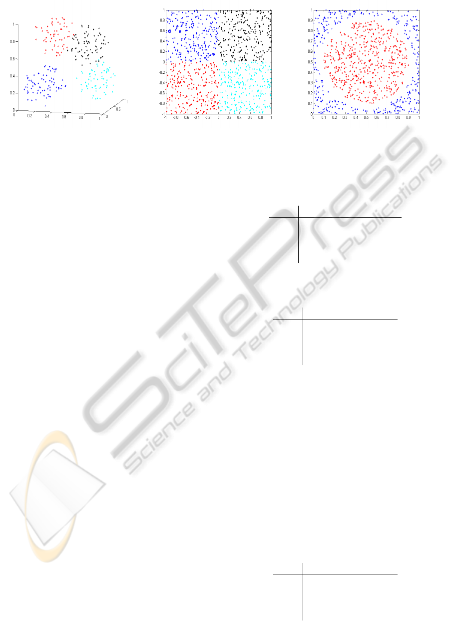
(a) (b) (c)
Figure 1: Illustration of the three first artificial problems; (a) Spheres, (b) Squares, (c) Circle.
5.2 Artificial Problems
The three strategies described above are first com-
pared on five artificial data sets, for which the relevant
features are known.
The first one is called the spheres prob-
lem. It consists in dividing the data points
into four classes corresponding to four spheres
of radius 0.25 and centered respectively in
(0.25, 0.25, 0.25), (0.25, 0.75, 0.75), (0.75, 0.75, 0.25)
and (0.75, 0.25, 0.75). A data set composed of 6
features uniformly distributed between 0 and 1 is
built; only the three first ones, used as coordinates in
a three-dimensional space, are useful to define the
class labels. The sample size is 50.
The second problem, called squares, consists in
four classes defined according to four contiguous
squares whose size length is 1. Again, 6 features uni-
formly distributed between 0 and 1 are built while
only the first two serve as coordinates in a two-
dimensional space and are relevant to discriminate be-
tween the classes. The sample size is 100.
The third artificial problem, denoted circle, is a bi-
nary classification one. A circle of radius 0.4 is set at
the center of a square of size length 1 and two classes
are defined according to whether or not a point lies in-
side the circle. A ring of width 0.05 separates the two
classes. Only the first two features are thus relevant in
this case; the sample size is 500. Figure 1 represents
the three first articial problems.
The fourth and fifth problems both have 10 fea-
tures f
1
. . . f
10
and a sample size of 300. The class
labels are generated by discretizing the following out-
puts:
Y
4
= cos(2 f
1
)cos( f
3
)exp(2 f
3
)exp(2 f
4
) (11)
and
Y
5
= 10 sin( f
1
f
2
)+20( f
3
−0.5)
2
+10 f
4
+5 f
5
, (12)
Table 1: Percentage of relevant features obtained by the
three feature selection techniques on the spheres data set.
µ WLS y
max
y
error
0.3 100 99.33 96.67
0.35 98 93.33 92
0.4 97.33 90 88.67
0.45 91.33 80 80
Table 2: Percentage of relevant features obtained by the
three feature selection techniques on the squares data set.
µ WLS y
max
y
error
0.35 100 98 96
0.4 99 94 96
0.45 99 93 90
0.5 96 81 78
this last problem being derived from (Friedman,
1991). More precisely, the sample points are first
ranked in increasing value of Y
4
or Y
5
. They are then
respectively divided into three and two classes con-
taining the same number of consecutive points.
To compare the different feature selection strate-
gies, the criterion is the percentage of relevant fea-
tures among the n
r
best ranked features, with n
r
being
the total number of relevant features for a given prob-
lem. All the artificial data sets have been randomly
generated 50 times to repeat the experiments. [!ht]
Tables 1 to 5 present the results obtained with var-
Table 3: Percentage of relevant features obtained by the
three feature selection techniques on the circles data set.
µ WLS y
max
y
error
0.25 100 100 92
0.30 97 97 87
0.35 89 85 74
0.40 80 72 64
ICPRAM 2012 - International Conference on Pattern Recognition Applications and Methods
166
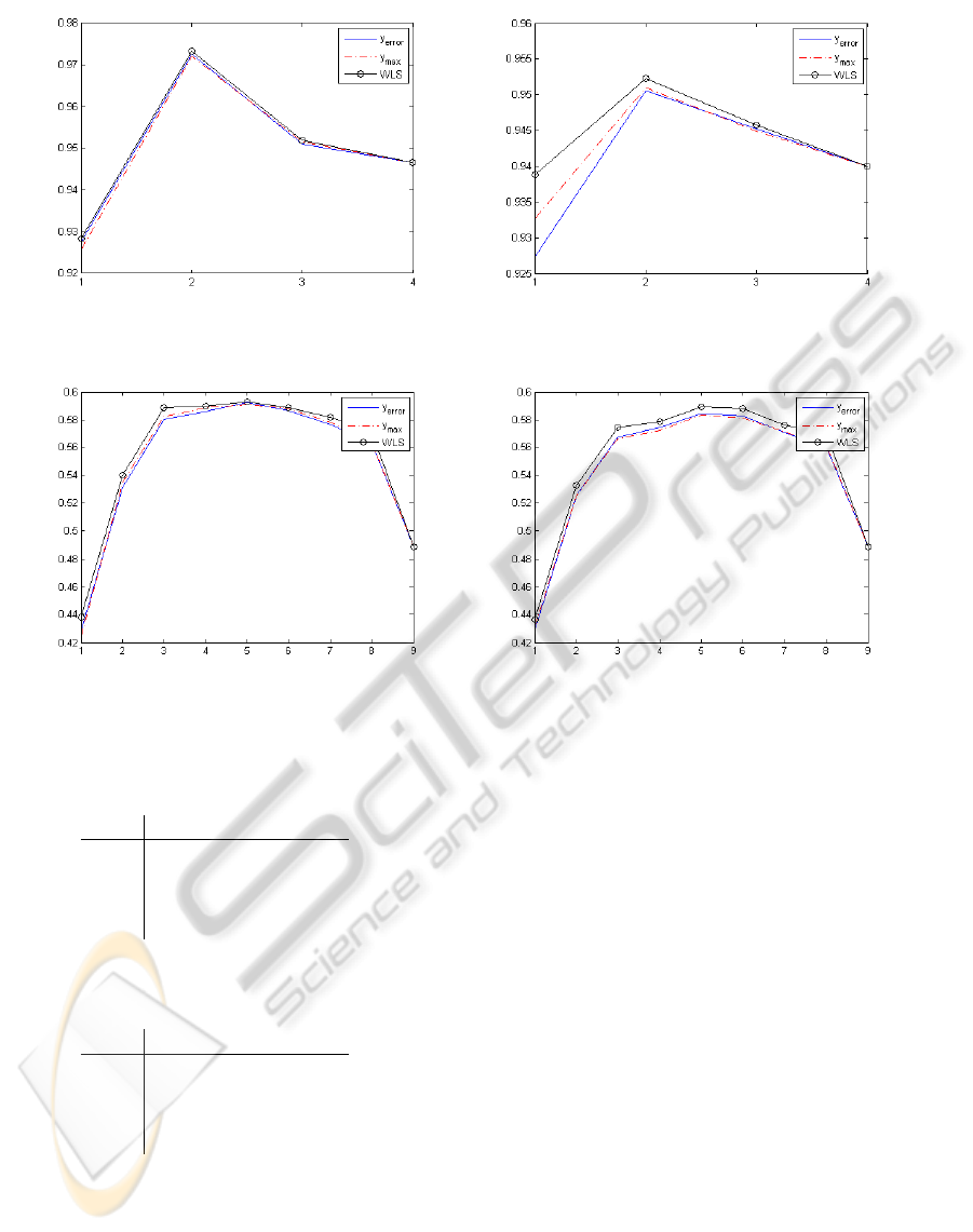
Figure 2: Accuracy of a 1NN classifier as a function of the number of selected features for the Iris data set with µ = 0.2 (left)
and µ = 0.3 (right).
Figure 3: Accuracy of a 1NN classifier as a function of the number of selected features for the Breast Tissue data set with
µ = 0.2 (left) and µ = 0.3 (right).
Table 4: Percentage of relevant features obtained by the
three feature selection techniques on the Y
4
data set.
µ WLS y
max
y
error
0.25 95.5 94.5 88.5
0.30 95 89 87
0.35 89.5 82.5 82
0.40 84.5 75 74
Table 5: Percentage of relevant features obtained by the
three feature selection techniques on the Y
5
data set.
µ WLS y
max
y
error
0.25 96.8 93.6 91.6
0.30 94 90 84.8
0.35 84.8 79.2 74.4
0.40 76.4 72.4 59.6
ious values of µ, depending on the complexity of the
problem. The results obtained on the five considered
artificial problems lead to very similar conclusions.
Indeed, for each problem and each value of µ, the pro-
posed WLS always outperforms its two competitors
by more accurately detecting the relevant features.
Moreover, the WLS performances are very satisfac-
tory since, for example, it selects on average more
than 90% of relevant features when µ = 0.3. This in-
dicates the adequateness of the proposed feature se-
lection strategy for problems with uncertain labels.
As could be expected, the differences in perfor-
mance between the methods are slightly smaller when
µ remains low. However, when µ is raised to more
than 25% or 30%, the advantage of considering the
uncertainty for feature selection appears clearly. As
an example, one can notice that for the spheres data
set, WLS selects 7.33% and 11.33% more relevant
features than the y
max
based strategy for respectively
µ = 35% and µ = 45%. This difference in perfor-
mances increases to 15% on the squares data set when
µ = 50%. Generally, the method based on the ob-
served class labels y
error
performs the worse.
5.3 Real-world Data Sets
To further assess the interest of the proposed feature
scoring criterion, experiments are also carried out on
three real-world data sets. The first one is the well
known Iris data set, whose objective is to assign each
sample to one of three iris types, based on four fea-
HANDLING IMPRECISE LABELS IN FEATURE SELECTION WITH GRAPH LAPLACIAN
167

Figure 4: Accuracy of a 1NN classifier as a function of the number of selected features for the Mines data set with µ = 0.2
(left) and µ = 0.3 (right).
tures. The sample size is 150. The second data set is
called Breast Tissue; it contains 106 samples and ten
features. The goal is to classify breast tissues into four
possible classes. The third data set is called Mines vs.
Rocks. The objective is to decide whether a sonar sig-
nal was bounced off by a metal cylinder (a mine) or
by a rock based on 60 features corresponding to the
energy within a particular frequency band. The sam-
ple size is 208. These three data sets can be obtained
from the UCI Machine Learning Repository website
(Asuncion and Newman, 2007).
Since the most relevant features are not known in
advance for these three data sets, the comparison cri-
terion will be the accuracy of a classifier using the fea-
tures selected by the three methods. More precisely,
a 1-nearest neighbors (1NN) classifier will be used,
as it is kwown to suffer dramatically from the pres-
ence of irrelevant features. The exact class labels will
be used for the classification step while, as has been
done before, the feature selection will be achieved
with the possibly permuted labels and the expert in-
formation. This way the ability of the methods to se-
lect relevant features for the true original problem can
be compared.
Figures 2, 3 and 4 present the accuracy of the 1NN
classifier as a function of the number of selected fea-
tures for µ = 20% and µ = 30%. For each data set
and each µ, the label permutation phase is randomly
repeated 50 times and the results are obtained as an
average over a five-fold cross validation procedure.
The results confirm the interest of the proposed
W LS. Indeed, for the Iris and the Breast Tissue data
sets, the WLS leads to better or equal classification
performances than its two competitors for any num-
ber of features and both contamination rates. The
differences in performance are of course larger when
µ = 30%. The Mines data set also confirms that the
W LS is able to detect relevant features more quickly
than the methods which do not take label uncertainty
into account. As can be seen in Figure 4, WLS out-
perfoms the other two approaches for the first 12 and
the first 16 features when µ equals 20% and 30% re-
spectively. In both cases, it leads to a global best clas-
sification accuracy.
6 CONCLUSIONS
This paper proposes a way to achieve feature selec-
tion for classification problems with imprecise labels.
More precisely, problems for which each class label
is associated with a probability value for each sample
are considered. Such problems can result from the
hesitation of an expert anotating the samples or from
the combination of several experts’ opinion; they are
likely to be encountered when a human supervision is
required to assign a class label to the points of a data
set and is thus important to consider in practice. In-
deed, such situations are frequently encountered for
medical or text categorisation problems (among oth-
ers) where errors are also possible.
The suggested methodology is based on the theory
of graph Laplacian, which received a great amount of
interest for feature selection the last few years. The
idea is to rank the features according to their ability
to preserve a neighborhood relationship defined be-
tween samples. In this paper, this relationship is de-
fined by computing the probabilities that two points
share the same class label. Obviously, the exact same
methodology could as well be applied for problems
where only one possible label is given with a measure
of the confidence about the accuracy of this label.
Experiments on both artificial and real-world data
sets have clearly demonstrated the interest of the pro-
posed approach when compared with methods also
based on Graph laplacian that do not take the label
uncertainty into account.
ICPRAM 2012 - International Conference on Pattern Recognition Applications and Methods
168

ACKNOWLEDGEMENTS
Gauthier Doquire is funded by a Belgian F.R.I.A.
grant.
REFERENCES
Asuncion, A. and Newman, D. (2007). UCI machine learn-
ing repository. University of California, Irvine, School
of Information and Computer Sciences, available at
http://www.ics.uci.edu/∼mlearn/MLRepository.html.
Bezdez, J. C. and Pal, S. K. (1992). Fuzzy models for pat-
tern recognition. IEEE Press, Piscataway, NJ.
Chapelle, O., Sch
¨
olkopf, B., and Zien, A., editors (2006).
Semi-Supervised Learning. MIT Press, Cambridge,
MA.
Chung, F. R. K. (1997). Spectral Graph Theory (CBMS
Regional Conference Series in Mathematics, No. 92).
American Mathematical Society.
C
ˆ
ome, E., Oukhellou, L., Denoeux, T., and Aknin, P.
(2009). Learning from partially supervised data using
mixture models and belief functions. Pattern Recogn.,
42:334–348.
Dash, M. and Liu, H. (1997). Feature selection for classifi-
cation. Intelligent Data Analysis, 1:131–156.
Denoeux, T. and Zouhal, L. M. (2001). Handling possi-
bilistic labels in pattern classification using evidential
reasoning. Fuzzy Sets and Systems, 122(3):47–62.
Ding, C. and Peng, H. (2003). Minimum redundancy fea-
ture selection from microarray gene expression data.
In Proceedings of the IEEE Computer Society Con-
ference on Bioinformatics, CSB ’03, pages 523–528,
Washington, DC, USA. IEEE Computer Society.
Friedman, J. H. (1991). Multivariate adaptive regression
splines. The Annals of Statistics, 19(1):1–67.
Guyon, I. and Elisseeff, A. (2003). An introduction to
variable and feature selection. J. Mach. Learn. Res.,
3:1157–1182.
Hall, M. (1999). Correlation-based Feature Selection for
Machine Learning. PhD thesis, University of Waikato.
He, X., Cai, D., and Niyogi, P. (2006). Laplacian Score
for Feature Selection. In Advances in Neural Infor-
mation Processing Systems 18, pages 507–514. MIT
Press, Cambridge, MA.
Jenhani, I., Amor, N. B., and Elouedi, Z. (2008). Decision
trees as possibilistic classifiers. Int. J. Approx. Rea-
soning, 48:784–807.
Kohavi, R. and John, G. H. (1997). Wrappers for Feature
Subset Selection. Artificial Intelligence, 97:273–324.
Kwak, N. and Choi, C.-H. (2002). Input feature selec-
tion for classification problems. IEEE Transactions
on Neural Networks, 13:143–159.
Meyer, P. E., Schretter, C., and Bontempi, G. (2008).
Information-Theoretic Feature Selection in Microar-
ray Data Using Variable Complementarity. Se-
lected Topics in Signal Processing, IEEE Journal of,
2(3):261–274.
Peng, H., Long, F., and Ding, C. (2005). Feature se-
lection based on mutual information criteria of max-
dependency, max-relevance, and min-redundancy.
IEEE Transactions on Pattern Analysis and Machine
Intelligence, 27(8):1226–1238.
Semani, D., Fr
´
elicot, C., and Courtellemont, P. (2004).
Combinaison d’
´
etiquettes floues/possibilistes pour la
s
´
election de variables. In 14ieme Congr
`
es Franco-
phone AFRIF-AFIA de Reconnaissance des Formes et
Intelligence Artificielle, RFIA’04, pages 479–488.
Smets, P., Hsia, Y., Saffiotti, A., Kennes, R., Xu, H.,
and Umkehren, E. (1991). The transferable belief
model. Symbolic and Quantitative Approaches to Un-
certainty, pages 91–96.
Tibshirani, R. (1996). Regression shrinkage and selection
via the lasso. Journal of the Royal Statistical Society
B, 58:267–288.
Wang, B., Jia, Y., Han, Y., and Han, W. (2009). Effective
feature selection on data with uncertain labels. In Pro-
ceedings of the 2009 IEEE International Conference
on Data Engineering, pages 1657–1662, Washington,
DC, USA.
Yang, Y. and Pedersen, J. O. (1997). A comparative study
on feature selection in text categorization. In Pro-
ceedings of the Fourteenth International Conference
on Machine Learning, ICML ’97, pages 412–420, San
Francisco, CA, USA. Morgan Kaufmann Publishers
Inc.
Yuan, M. and Lin, Y. (2006). Model selection and estima-
tion in regression with grouped variables. Journal of
the Royal Statistical Society, Series B, 68:49–67.
Zhang, D., Chen, S., and Zhou, Z.-H. (2008). Constraint
score: A new filter method for feature selection with
pairwise constraints. Pattern Recogn., 41:1440–1451.
Zhao, J., Lu, K., and He, X. (2008). Locality sensitive
semi-supervised feature selection. Neurocomputing,
71:1842–1849.
Zhao, Z. and Liu, H. (2007). Semi-supervised Feature Se-
lection via Spectral Analysis. In Proceedings of the
7th SIAM International Conference on Data Mining.
HANDLING IMPRECISE LABELS IN FEATURE SELECTION WITH GRAPH LAPLACIAN
169
