
DYNAMICALLY MIXING DYNAMIC LINEAR MODELS WITH
APPLICATIONS IN FINANCE
Kevin R. Keane and Jason J. Corso
Department of Computer Science and Engineering
University at Buffalo, The State University of New York, Buffalo, NY, U.S.A.
Keywords:
Bayesian inference, Dynamic linear models, Multi-process models, Statistical arbitrage.
Abstract:
Time varying model parameters offer tremendous flexibility while requiring more sophisticated learning meth-
ods. We discuss on-line estimation of time varying DLM parameters by means of a dynamic mixture model
composed of constant parameter DLMs. For time series with low signal-to-noise ratios, we propose a novel
method of constructing model priors. We calculate model likelihoods by comparing forecast distributions
with observed values. We utilize computationally efficient moment matching Gaussians to approximate exact
mixtures of path dependent posterior densities. The effectiveness of our approach is illustrated by extracting
insightful time varying parameters for an ETF returns model in a period spanning the 2008 financial crisis.
We conclude by demonstrating the superior performance of time varying mixture models against constant
parameter DLMs in a statistical arbitrage application.
1 BACKGROUND
1.1 Linear Models
Linear models are utilitarian work horses in many do-
mains of application. A model’s linear relationship
between a regression vector F
t
and an observed re-
sponse Y
t
is expressed through coefficients of a re-
gression parameter vector θ. Allowing an error of fit
term ε
t
, a linear regression model takes the form:
Y = F
T
θ+ ε , (1)
where Y is a column vector of individual observations
Y
t
, F is a matrix with column vectors F
t
correspond-
ing to individual regression vectors, and ε a column
vector of individual errors ε
t
.
The vector Y and the matrix F are observed. The
ordinary least squares (“OLS”) estimate
ˆ
θ of the re-
gression parameter vector θ is (Johnson and Wichern,
2002):
ˆ
θ =
FF
T
−1
FY . (2)
1.2 Stock Returns Example
In modeling the returns of an individual stock, we
might believe that a stock’s return is roughly a linear
function of market return, industry return, and stock
specific return. This could be expressed as a linear
model in the form of (1) as follows:
r = F
T
θ+ ε, F =
1
r
M
r
I
, θ =
α
β
M
β
I
, (3)
where r represents the stock’s return, r
M
is the market
return, r
I
is the industry return, α is a stock specific
return component, β
M
is the sensitivity of the stock to
market return, and β
I
is the sensitivity of the stock to
it’s industry return.
1.3 Dynamic Linear Models
Ordinary least squares, as defined in (2), yields a sin-
gle estimate
ˆ
θ of the regression parameter vector θ
for the entire data set. Problems arise with this frame-
work if we don’t have a finite data set, but rather an in-
finite data stream. We might expect θ, the coefficients
of a linear relationship, to vary slightly over time
θ
t
≈θ
t+1
. This motivates the introduction of dynamic
linear models (West and Harrison, 1997). DLMs are a
generalized form, subsuming Kalman filters (Kalman
et al., 1960), flexible least squares (Kalaba and Tesfat-
sion, 1996), linear dynamical systems (Minka, 1999;
Bishop, 2006), and several time series methods —
Holt’s point predictor, exponentially weighted mov-
ing averages, Brown’s exponentially weighted regres-
295
R. Keane K. and J. Corso J. (2012).
DYNAMICALLY MIXING DYNAMIC LINEAR MODELS WITH APPLICATIONS IN FINANCE.
In Proceedings of the 1st International Conference on Pattern Recognition Applications and Methods, pages 295-302
DOI: 10.5220/0003712602950302
Copyright
c
SciTePress

sion, and Box-Jenkins autoregressive integrated mov-
ing average models (West and Harrison, 1997). The
regime switching model in (Hamilton, 1994) may
be expressed as a DLM, specifying an autoregres-
sive model where evolution variance is zero except
at times of regime change.
1.4 Contributions and Paper Structure
The remainder of the paper is organized as follows.
In section §2, we introduce DLMs in further detail;
discuss updating estimated model parameter distri-
butions upon arrival of incremental data; show how
forecast distributions and forecast errors may be used
to evaluate candidate models; the generation of data
given a DLM specification; inference as to which
model was the likely generator of the observed data;
and, a simple example of model inference using syn-
thetic data with known parameters. Building upon
this base, in section §3 multi-process mixture mod-
els are introduced. We report design challenges we
tackled in implementing a mixture model for finan-
cial time series. In section §4, we introduce an al-
ternative set of widely available financial time series
permitting easier replication of the work in (Montana
et al., 2009); and we provide an example of apply-
ing a mixture model to real world financial data, ex-
tracting insightful time varying estimates of variance
in an ETF returns model during the recent financial
crisis. In section §5, we augment the statistical ar-
bitrage strategy proposed in (Montana et al., 2009)
by incorporating a hedge that significantly improves
strategy performance. We demonstrate that an on-line
dynamic mixture model outperforms all statically pa-
rameterized DLMs. Further, we draw attention to the
fact that the period of unusually large mispricing iden-
tified by our mixture model coincides with unusually
high profitability for the statistical arbitrage strategy.
In §6, we conclude.
2 DYNAMIC LINEAR MODELS
2.1 Specifying a DLM
In the framework of (West and Harrison, 1997), a
dynamic linear model is specified by its parameter
quadruple {F
t
,G,V,W}. DLMs are controlled by two
key equations. One is the observation equation:
Y
t
= F
T
t
θ
t
+ ν
t
, ν
t
∼ N(0,V) , (4)
the other is the evolution equation:
θ
t
= Gθ
t−1
+ ω
t
, ω
t
∼ N(0,W) . (5)
Algorithm 1: Updating a DLM given G,V,W.
Initialize t = 0
{Initial information p(θ
0
|D
0
) ∼ N[m
0
,C
0
]}
Input: m
0
, C
0
, G, V, W
loop
t = t + 1
{Compute prior at t: p(θ
t
|D
t−1
) ∼ N[a
t
,R
t
]}
a
t
= Gm
t−1
R
t
= GC
t−1
G
T
+W
Input: F
t
{Compute forecast at t: p(Y
t
|D
t−1
) ∼ N[f
t
,Q
t
]}
f
t
= F
T
t
a
t
Q
t
= F
T
t
R
t
F
t
+V
Input: Y
t
{Compute forecast error e
t
}
e
t
= Y
t
− f
t
{Compute adaptive vector A
t
}
A
t
= R
t
F
t
Q
−1
t
{Compute posterior at t: p(θ
t
|D
t
) ∼ N[m
t
,C
t
]}
m
t
= a
t
+ A
t
e
t
C
t
= R
t
−A
t
Q
t
A
T
t
end loop
F
T
t
is a row in the design matrix representing inde-
pendent variables effecting Y
t
. G is the evolution
matrix, capturing deterministic changes to θ, where
θ
t
≈ Gθ
t−1
. V is the observational variance, Var(ε)
in ordinary least squares. W is the evolution vari-
ance matrix, capturing random changes to θ, where
θ
t
= Gθ
t−1
+ w
t
, w
t
∼ N(0,W). The two parame-
ters G and W make a linear model dynamic.
2.2 Updating a DLM
The Bayesian nature of a DLM is evident in the care-
ful accounting of sources of variation that generally
increase system uncertainty; and, information in the
form of incremental observations that generally de-
crease system uncertainty. A DLM starts with initial
information, summarized by the parameters of a (fre-
quently multivariate) normal distribution:
p(θ
0
|D
0
) ∼ N (m
0
,C
0
) . (6)
At each time step, the information is augmented as
follows:
D
t
= {Y
t
,D
t−1
} . (7)
Algorithm 1 details the relatively simple steps of
updating a DLM as additional regression vectors F
t
and observationsY
t
become available. Note that upon
arrival of the current regression vector F
t
, a one-step
forecast distribution p(Y
t
|D
t−1
) is computed using the
prior distribution p(θ
t
|D
t−1
), the regression vector F
t
,
and the observation noise V.
ICPRAM 2012 - International Conference on Pattern Recognition Applications and Methods
296
2.3 Model Likelihood
The one-step forecast distribution facilitates compu-
tation of model likelihood by evaluation of the den-
sity of the one-step forecast distribution p(Y
t
|D
t−1
)
for observation Y
t
. The distribution p(Y
t
|D
t−1
) is ex-
plicitly a function of the previous periods informa-
tion D
t−1
; and, implicitly a function of static model
parameters {G,V,W} and model state determined by
a series of updates resulting from the history D
t−1
.
Defining a model at time t as M
t
= {G,V,W, D
t−1
},
and explicitly displaying the M
t
dependency in the
one-step forecast distribution, we see that the one-
step forecast distribution is equivalent to model like-
lihood
1
:
p(Y
t
|D
t−1
) = p(Y
t
,D
t−1
|D
t−1
,M
t
) = p(D
t
|M
t
) (8)
Model likelihood, p(D
t
|M
t
), will be an important in-
put to our mixture model discussed below.
0 200 400 600 800 1000
−10
0
10
20
30
Time t
Observed Data Y
t
W=.05
W=5 W=.0005
DLM {1,1,1,W}
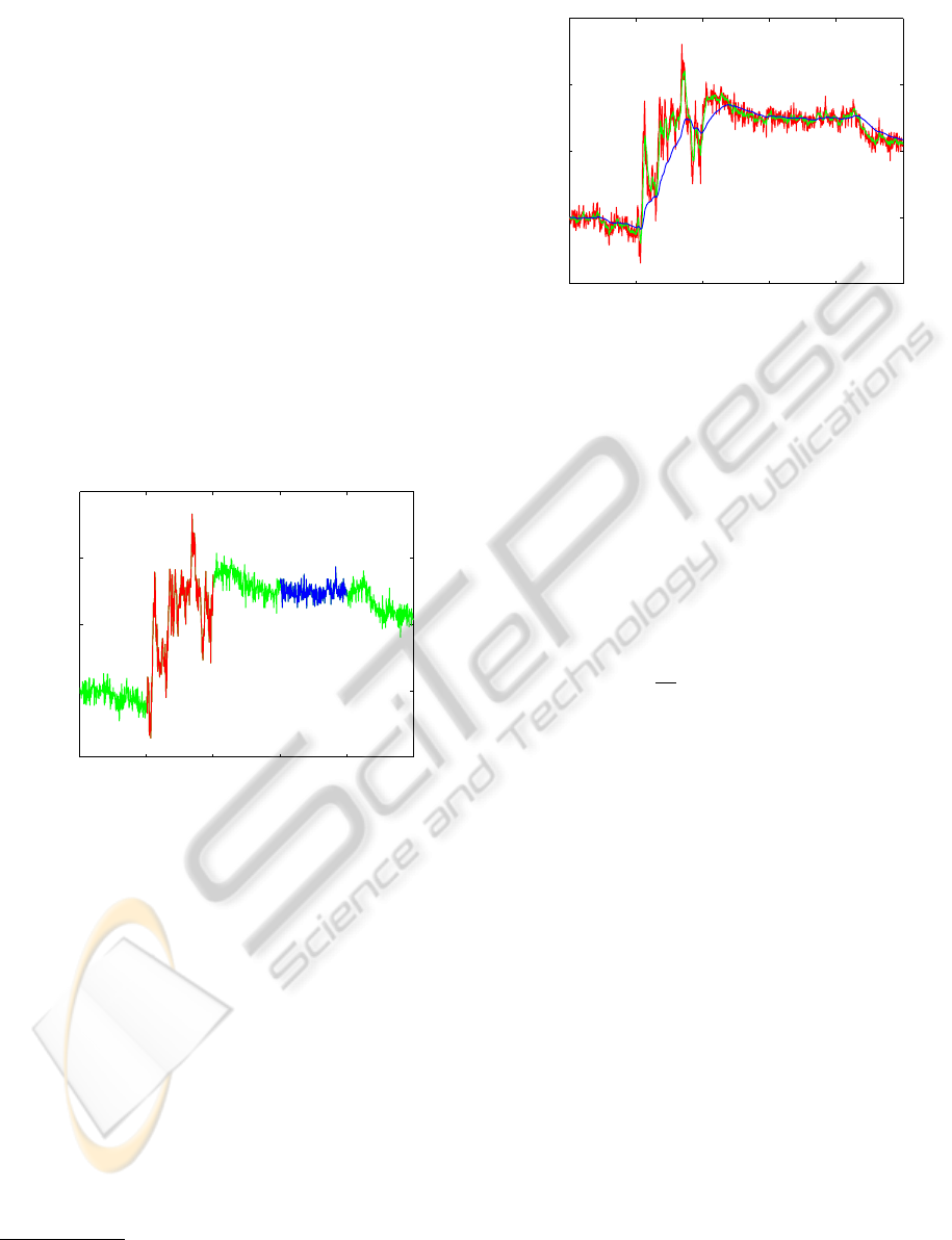
Figure 1: Observations Y
t
generated from a mixture of three
DLMs. Discussion appears in §2.4
2.4 Generating Observations
Before delving into mixtures of DLMs, we illustrate
the effect of varying the evolution variance W on the
state variable θ in a very simple DLM. In Figure 1
we define three very simple DLMs, {1,1,1,W
i
},W
i
∈
{.0005,.05,5}. The observations are from simple
random walks, where the level of the series θ
t
varies
according to an evolution equation θ
t
= θ
t−1
+ω
t
, and
the observation equation is Y
t
= θ
t
+ ν
t
. Compare the
relative stability in the level of observations generated
by the three models. Dramatic and interesting behav-
ior materializes as W increases.
1
D
t
= {Y
t
,D
t−1
} by definition; M
t
contains
D
t−1
by definition; and, p(Y
t
,D
t−1
|D
t−1
) =
p(Y
t
|D
t−1
)p(D
t−1
|D
t−1
) = p(Y
t
|D
t−1
).
0 200 400 600 800 1000
−10
0
10
20
30
Time t
m
t
W=5
W=.05
W=.0005
DLM {1,1,1,W}
Figure 2: Estimates of the mean of the state variable θ
t
for
three DLMs when processing generated data of Figure 1.
2.5 Model Inference
Figure 1 illustrated the differencein appearance of ob-
servations Y
t
generated with different DLM parame-
ters. In Figure 2, note that models with smaller evo-
lution variance W result in smoother estimates — at
the expense of a delay in responding to changes in
level. At the other end of the spectrum, large W per-
mits rapid changes in estimates of θ — at the ex-
pense of smoothness. In terms of the model likeli-
hood p(D
t
|M
t
), if W is too small, the standardized
forecast errors e
t
/
√
Q
t
will be large in magnitude, and
therefore model likelihood will be low. At the other
extreme, if W is too large, the standardized forecast
errors will appear small, but the model likelihood will
be low now due to the diffuse forecast distribution.
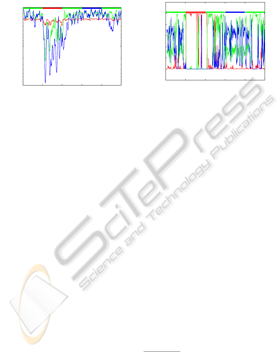
In Figure 3, we graph the trailing interval log like-
lihoods for each of the three DLMs. We define trailing
interval (k-period) likelihood as:
L
t
(k) = p(Y
t
,Y
t−1
,...,Y
t−k+1
|D
t−k
)
= p(Y
t
|D
t−1
)p(Y
t−1
|D
t−2
)...
p(Y
t−k+1
|D
t−k
) .
(9)
This concept is very similar to Bayes’ factors dis-
cussed in (West and Harrison, 1997), although we
do not divide by the likelihood of an alternative
model. Our trailing interval likelihood is also simi-
lar to the likelihood function discussed in (Crassidis
and Cheng, 2007); but, we assume the errors e
t
are
not autocorrelated.
Across the top of Figure 3 appears a color code
indicating the true model prevailing at time t. It is
interesting to note when the likelihood of a model ex-
ceeds that of the true model. For instance, around the
t = 375 mark, the model with the smallest evolution
variance appears most likely. Reviewing Figure 2,
the state estimates of DLM {1,1,1,W = .0005} just
DYNAMICALLY MIXING DYNAMIC LINEAR MODELS WITH APPLICATIONS IN FINANCE
297
0 200 400 600 800 1000
−10
3
−10
2
−10
1
Time t
10−day log likelihood
W=5 W=.05 W=.0005
Figure 3: Log likelihood of observed data during most re-
cent 10 days given the parameters of three DLMs when pro-
cessing generated data of Figure 1. Bold band at top of fig-
ure indicates the true generating DLM.
happened to be in the right place at the right time.
Due to the more concentrated forecast distributions
p(Y
t
|D
t−1
) of this model, it briefly attains the high-
est trailing 10-period log likelihood. A similar oc-
currence can be seen for the DLM {1, 1,1,W = .05}
around t = 325.
While the series on Figure 3 appear visually close
at times, note the log scale. After converting back to
normalized model probabilities, the favored model at
a particular instance is more apparent as illustrated in
Figure 4. In §5, we will perform model inference on
the return series of exchange traded funds (ETFs).
3 PARAMETER ESTIMATION
In §2, we casually discussed DLMs varying in pa-
rameterization. Generating observations from a spec-
ified DLM or combination of DLMs, as in §2.4, is
trivial. The inverse problem, determining model pa-
rameters from observations is significantly more chal-
lenging. There are two distinct versions of this task
based upon area of application. In the simpler case,
the parameters are unknown but assumed constant. A
number of methods are available for model identifi-
cation in this case, both off-line and on-line. For ex-
ample, (Ghahramani and Hinton, 1996) use E-M off-
line, and (Crassidis and Cheng, 2007) use the likeli-
hood of a fixed-length trailing window of prediction
errors on-line. Time varying parameters are signifi-
cantly more challenging. The posterior distributions
are path dependent and the number of paths is expo-
nential in the length of the time series. Various ap-
proaches are invoked to obtain approximate solutions
with reasonable computational effort. (West and Har-
0 200 400 600 800 1000
−0.2
0
0.2
0.4
0.6
0.8
1
Time t
P( M | D )
W=5 W=.05 W=.0005
Figure 4: Model probabilities from normalized likelihoods
of observed data during most recent 10 periods. Bold band
at top of figure indicates the true generating DLM.
rison, 1997) approximate the posterior with a single
Gaussian that matches the moments of the exact dis-
tribution. (Valpola et al., 2004; Sarkka and Nummen-
maa, 2009) propose variational Bayesian approxima-
tion. (Minka, T.P., 2007) discusses Gaussian-sum and
assumed-density filters.
3.1 Multi-process Mixture Models
(West and Harrison, 1997) define sets of DLMs,
where the defining parameters M
t
= {F, G,V,W}
t
are
indexed by λ
2
, so that M
t
= M(λ
t
). The set of DLMs
at time t is {M(λ
t
) : λ
t
∈ Λ}. Two types of multi-
process models are defined. A class I multi-process
model, where for some unknown λ
0
∈Λ,M(λ
0
) holds
for all t; and, a class II multi-process model for some
unknown sequence λ
t
∈ Λ,(t = 1, 2,...),M(λ
t
) holds
at time t. We build our model in §4 in the framework
of a class II mixture model. We do not expect to be
able to specify parameters exactly or finitely. Instead,
we specify a set of models that quantize a range of
values. In the terminology of (Sarkka and Nummen-
maa, 2009), we will create a grid approximation to
the evolution and observation variance distributions.
Class II mixture models permit the specification
of a model per time period, leading to a number of
potential model sequences exponential in the steps,
|Λ|
T
. However, in the spirit of the localized nature of
dynamic models and practicality, (West and Harrison,
1997) exploit the fact that the value of information
decreases quickly with time, and propose collapsing
2
(West and Harrison, 1997) index the set of component
models α ∈ A ; however, by convention in finance, α refers
to stock specific return, consistent with §1.2. To avoid con-
fusion, we index the set of component models λ ∈ Λ, con-
sistent with the notation of (Chen and Liu, 2000).
ICPRAM 2012 - International Conference on Pattern Recognition Applications and Methods
298

the paths and approximating common posterior dis-
tributions. In the filtering literature, this technique is
referred to as the interacting multiple model (IMM)
estimator (Bar-Shalom et al., 2001, Ch. 11.6.6). In
our application, in §5, we limit our sequences to two
steps, and approximate common posterior distribu-
tions by collapsing individual paths based on the most
recent two component models. To restate this briefly,
we model two step sequences — the component
model M
t−1
just exited, and the component model M
t
now occupied. Thus, we consider |Λ|
2
sequences. Re-
viewing Algorithm 1, the only information required
from t −1 is captured in the collapsed approximate
posterior distribution p(θ
t−1
|D
t−1
) ∼ N (m
t−1
,C
t−1
)
for each component model λ
t−1
∈ Λ considered.
3.2 Specifying Model Priors
One key input to mixture models are the model pri-
ors. We have tried several approaches to this task
before finding a method suitable for our statistical
arbitrage modeling task in §5. The goal of our en-
tire modeling process is to design a set of model
priors p(M(λ
t
)) and model likelihoods p(D|M(λ
t
))
that yield in combination insightful model posterior
distributions p(M(λ
t
)|D), permitting the computation
of quantities of interest by summing over the model
space λ
t
∈ Λ at time t:
p(X
t
|D
t
) ∝
∑
λ
t
∈Λ
p(X
t
|M(λ
t
))p(M(λ
t
)|D
t
) (10)
In the context of modeling ETF returns discussed
in §5, the vastly different scales for the contribu-
tion of W and V to Q left our model likelihoods un-
responsive to values of W. This unresponsiveness
was due to the fact that parameter values W and V
are of similar scale; however, a typical |F
t
| for this
model is approximately 0.01, and therefore the re-
spective contributions to the forecast variance Q =
F
T
RF +V = F
T
(GCG
T
+ W)F + V are of vastly dif-
ferent scales, 1 : 10,000. Specifically, density of the
likelihood p(Y
t
|D
t−1
) ∼ N(f
t
,Q
t
) is practically con-
stant for varying W after the scaling by 0.01
2
. The
only knob left for us to twist is that of the model pri-
ors.
DLMs with static parameters embed evidence of
recent model relevance in their one-step forecast dis-
tributions. In contrast, mixture model component
DLMs move forward in time from posterior distribu-
tions that mask model performance. The situation is
similar to the game best ball in golf. After each player
hits the ball, all players’ balls are moved to a best po-
sition as a group. Analogously, when collapsing pos-
terior distributions, sequences originating from differ-
ent paths are approximated with a common posterior
based upon end-point model. While some of us may
appreciate obfuscation of our golf skills, the obfus-
cation of model performance is problematic. Due to
the variance scaling issues of our application, the path
collapsing, common posterior density approximating
technique destroys the accumulation of evidence in
one-step forecast distributions for specific DLM pa-
rameterizations λ ∈ Λ. In our current implementa-
tion, we retain local evidence of model effectiveness
by running a parallel set of standalone (not mixed)
DLMs. Thus, the total number of models maintained
is |Λ|
2
+ |Λ|, and the computational complexity re-
mains asymptotically constant. In our mixture model,
we define model priors proportional to trailing in-
terval likelihoods from the standalone DLMs. This
methodology locally preserves evidence for individ-
ual models as shown in Figure 3 and Figure 4.
The posterior distributions p(θ
t
|D
t
)
M(λ)
emitted
by identically parameterized standalone and compo-
nent DLMs differ in general. A standalone constant
parameter DLM computes the prior p(θ
t
|D
t−1
)
M(λ
t
)
as outlined in Algorithm 1 using its own poste-
rior p(θ
t−1
|D
t−1
)
M(λ
t
=λ
t−1
)
. In contrast, component
DLMs compute prior distributions using a weighted
posterior:
p(θ
t−1
|D
t−1
)
M(λ
t
)
=
∑
λ
t−1
p(M(λ
t−1
)|M(λ
t
))p(θ
t−1
|D
t−1
)
M(λ
t−1
)
.
(11)
4 A FINANCIAL EXAMPLE
(Montana et al., 2009) proposed a model for the re-
turns of the S&P 500 Index based upon the largest
principal component of the underlying stock returns.
In the form Y = F
T
θ+ ε used throughout this paper,
Y = r
s&p
, F = r
pc1
, and θ = β
pc1
. (12)
The target and explanatory data in (Montana et al.,
2009) spanned January 1997 to October 2005. We
propose the use of two alternative price series that are
very similar in nature; but, publicly available, widely
disseminated, and tradeable. The proposed alterna-
tive to the S&P Index is the SPDR S&P 500 ETF
(trading symbol SPY). SPY is an ETF designed to
mimic the performance of the S&P 500 Index(PDR
Services LLC, 2010). The proposed alternative to the
largest principal component series is the Rydex S&P
Equal Weight ETF (trading symbol RSP). RSP is an
ETF designed to mimic the performance of the S&P
Equal Weight Index (Rydex Distributors, LLC, 2010).
While perhaps not as obvious a pairing as S&P Index /
DYNAMICALLY MIXING DYNAMIC LINEAR MODELS WITH APPLICATIONS IN FINANCE
299

2004 2006 2008 2010
50
100
150
200
250
Price
Date
RSP
SPY
Figure 5: SPDR S&P 500 (SPY) and Rydex S&P Equal
Weight (RSP) ETF closing prices, scaled to April 30, 2003
= 100.
SPY, a first principal component typically is the mean
of the data — in our context, the mean is the equal
weighted returns of the stocks underlying the S&P
500 Index. SPY began trading at the end of January
1993. RSP began trading at the end of April 2003.
We use the daily closing prices P
t
to compute daily
log returns:
r
t
= log
P
t
P
t−1
. (13)
Our analysis is based on the months during which
both ETFs traded, May 2003 to present (August
2011).
The price levels, scaled to 100 on April 30, 2003
are shown in Figure 5. Visually assessing the price
series, it appears the two ETFs have common direc-
tions of movement, with RSP displaying somewhat
greater range than SPY. Paralleling the work of (Mon-
tana et al., 2009), we will model the return of SPY as
a linear function of RSP, Y = F
T
θ+ ε:
Y = r
spy
, F = r
rsp
, and θ = β
rsp
. (14)
We estimate the time varying regression parameter
θ
t
using a class II mixture model composed of 50 can-
didate models with parameters {F
t
,1,V,W}. F
t
= r
rsp
,
the return of RSP, is common to all models. The
observation variances are the values V ×1,000, 000 ∈
{1, 2.15, 4.64, 10, 21.5, 46.4, 100, 215, 464, 1,000 }.
The evolution variances are the values
W × 1,000,000 ∈ { 10, 56, 320, 1,800, 10, 000 }.
Our on-line process computes 50
2
+ 50 = 2550
DLMs, 50
2
DLMs corresponding to the two-period
model sequences, and 50 standalone DLMs required
for trailing interval likelihoods. In the mixture
model, the priors p(M(λ
t
)) for component models
M(λ
t
), λ
t
∈ Λ, are proportional to trailing inter-
val likelihoods (9) of corresponding identically
parameterized standalone DLMs.
It’s an interesting side topic to consider the po-
tential scale of these mixtures. Circa 1989, in the
2004 2006 2008 2010
0.001
0.010
0.100
Std dev / day
Date
sqrt(V)
sqrt(W)
Figure 6: The daily standard deviation of ν
t
and ω
t
as
estimated by the mixture model. Observation noise ν
t
∼
N(0,V); evolution noise ω
t
∼ N(0,W).
predecessor text to (West and Harrison, 1997), West
and Harrison suggested the use of mixtures be re-
stricted for purposes of “computational economy”;
and that a single DLM would frequently be adequate.
Approximately one decade later, (Yelland and Lee,
2003) were running a production forecasting system
with 100 component models, and 10,000 model se-
quence combinations. Now, more than two decades
after West and Harrison’s practical recommendation,
with the advent of ubiquitous inexpensive GPGPUs,
the economics of computation have changed dramat-
ically. A direction of future research is to revisit im-
plementation of large scale mixture models quantiz-
ing several dimensions simultaneously.
Subsequent to running the mixture model for the
period May 2003 to present, we are able to review es-
timated time varying parameters V
t
and W
t
, as shown
in Figure 6. This graph displays the standard devia-
tion of observation and evolution noise, commonly re-
ferred to as volatility in the financial world. It is inter-
esting to review the decomposition of this volatility.
Whereas the relatively stationary series
√
W in Fig-
ure 6 suggests the rate of evolution of θ
t
is fairly con-
stant across time; the observation variance V varies
dramatically, rising noticeably during periods of fi-
nancial stress in 2008 and 2009. The observation vari-
ance, or standard deviation as shown, may be inter-
preted as the end-of-day mispricing of SPY relative
to RSP. In §5, we will demonstrate a trading strategy
taking advantage of this mispricing. The increased
observational variance at the end of 2008, visible in
Figure 6 results in an increase in the rate of profitabil-
ity of the statistical arbitrage application plainly visi-
ble in Figure 7.
5 STATISTICAL ARBITRAGE
(Montana et al., 2009) describe an illustrative statis-
ICPRAM 2012 - International Conference on Pattern Recognition Applications and Methods
300

2004 2006 2008 2010
0
50
100
% Return
Date
Best DLM {F,1,1,W=221}
DLMs {F,1,1,W}
Mixture Model
Figure 7: Cumulative return of the various implementations
of a statistical arbitrage strategy based upon a time varying
mixture model and 10 constant parameter DLMs.
tical arbitrage strategy. Their proposed strategy takes
equal value trading positions opposite the sign of the
most recently observed forecast error ε
t−1
. In the ter-
minology of this paper, they tested 11 constant param-
eter DLMs, with a parameterization variable δ equiv-
alent to:
δ =
W
W +V
. (15)
They note that this parameterization variable δ per-
mits easy interpretation. With δ ≈ 0, results ap-
proach an ordinary least squares solution: W = 0 im-
plies θ
t
= θ. Alternatively, as δ moves from 0 towards
1, θ
t
is increasingly permitted to vary.
Figure 6 challenges the concept that a constant
specification of evolution and observation variance
is appropriate for an ETF returns models. To ex-
plore the effectiveness of class II mixture models
versus statically parameterized DLMs, we evalu-
ated the performance of our mixture model against
10 constant parameter DLMs. We set V = 1 as
did (Montana et al., 2009), and specified W ∈
{29, 61,86,109,139, 179,221,280,412, 739}. These
values correspond to the 5, 15, ...95%-tile values of
W/V observed in our mixture model.
Figure 6 offers no justification of using V = 1.
While the prior p(θ
t
|D
t−1
), one-step p(Y
t
|D
t−1
) and
posterior p(θ
t
|D
t
) “distributions” emitted by these
DLMs will not be meaningful, the intent of such a
formulation is to provide time varying point estimates
of the state vector θ
t
. The distribution of θ
t
is not
of interest to modelers applying this approach. In the
context of the statistical arbitrage application consid-
ered here, the distribution is not required. The trading
rule proposed is based on the sign of the forecast er-
ror; and, the forecast is a function of the prior mean a
t
(a point estimate) for the state vector θ
t
and observed
values F
t
and Y
t
: ε
t
= Y
t
−F
T
t
a
t
.
10 100
2.0
2.5
3.0
Sharpe ratio
Evolution Variance W
DLMs {F,1,1,W}
Mixture Model
Figure 8: Sharpe ratios realized by the time varying mixture
model and 10 constant parameter DLMs.
5.1 The Trading Strategy
Consistent with (Montana et al., 2009), we ignore
trading and financing costs in this simplified experi-
ment. Given the setup of constant absolute value SPY
positions taken daily, we compute cumulative returns
by summing the daily returns. The rule we implement
is:
portfolio
t
(ε
t−1
) =
(
+1 if ε
t−1
≤ 0,
−1 if ε
t−1
> 0.
(16)
where
portfolio
t
= +1 denotes a long SPY and
short RSP position;
portfolio
t
= −1 denotes a short
SPY and long RSP position. The SPY leg of the trade
is of constant magnitude. The RSP leg is −a
t
× SPY-
value, where a
t
is the mean of the prior distribution of
θ
t
, p(θ
t
|D
t−1
) ∼ N(a
t
,R
t
); and, recall from (14) the
interpretation of θ
t
is the sensitivity of the returns of
SPY Y
t
to the returns of RSP F
t
. Note that this strat-
egy is a modification to (Montana et al., 2009) in that
we hedge the S&P exposure with the equal weighted
ETF, attempting to capture mispricings while elimi-
nating market exposure. The realized Sharpe ratios
appear dramatically higher in all cases than in (Mon-
tana et al., 2009), primarily attributable to the hedging
of market exposure in our variant of a simplified arbi-
trage example. Montana et al. report Sharpe ratios in
the 0.4 - 0.8 range; in this paper, after inclusion of the
hedging technique, Sharpe ratios are in the 2.3 - 2.6
range.
5.2 Analysis of Results
We reiterate that we did not include transaction costs
in this simple example. Had we done so, the results
would be significantly diminished. With that said, we
will review the relative performance of the models for
the trading application.
In Figure 7, it is striking that all models do fairly
DYNAMICALLY MIXING DYNAMIC LINEAR MODELS WITH APPLICATIONS IN FINANCE
301

well. The strategy holds positions based upon a com-
parison of the returns of two ETFs, one scaled by
an estimate of β
rsp
,t
. Apparently small variation in
the estimates of the regression parameter are not of
large consequence. Given the trading rule is based
on the sign of the error ε
t
, it appears that on many
days, slight variation in the estimate of θ
t
across
DLMs does not result in a change to
sign
(ε
t
). Fig-
ure 8 shows that over the interval studied, the mixture
model provided a higher return per unit of risk, if only
to a modest extent. What is worth mentioning is that
the comparison we make is the on-line mixture model
against the ex post best performance of all constant
parameter models. Acknowledging this distinction,
the mixture model’s performance is more impressive.
6 CONCLUSIONS
Mixtures of dynamic linear models are a useful tech-
nology for modeling time series data. We show the
ability of DLMs parameterized with time varying val-
ues to generate observations for complex dynamic
processes. Using a mixture of DLMs, we extract time
varying parameter estimates that offered insight to the
returns process of the S&P 500 ETF during the finan-
cial crisis of 2008. Our on-line mixture model demon-
strated superior performance compared to the ex post
optimal component DLM in a statistical arbitrage ap-
plication.
The contributions of this paper include the pro-
posal of a method, trailing interval likelihood, for
constructing component model prior probabilities.
This technique facilitated successful modeling of time
varying observational and evolution variance parame-
ters, and captured model evidence not adequately con-
veyed in the one-step forecast distribution due to scal-
ing issues. We proposed the use of two widely avail-
able time-series to facilitate easier replication and
extension of the statistical arbitrage application pro-
posed by (Montana et al., 2009). Our addition of
a hedge to the statistical arbitrage application from
(Montana et al., 2009) resulted in dramatically im-
proved Sharpe ratios.
We have only scratched the surface of the mod-
eling possibilities with DLMs. The mixture model
technique eliminates the burden of a priori specifica-
tion of process parameters. We look forward to evalu-
ating models with higher dimension state vectors and
parameterized evolution matrices. Due to the inher-
ently parallel nature of DLM mixtures, we also look
forward to exploring the ability of current hardware
to tackle additional challenging modeling problems.
REFERENCES
Bar-Shalom, Y., Li, X., Kirubarajan, T., and Wiley, J.
(2001). Estimation with applications to tracking and
navigation. John Wiley & Sons, Inc.
Bishop, C. (2006). Pattern Recognition and Ma-
chine Learning (Information Science and Statistics).
Springer Science+Business Media, LLC. New York,
NY, USA.
Chen, R. and Liu, J. (2000). Mixture Kalman filters. Jour-
nal of the Royal Statistical Society: Series B (Statisti-
cal Methodology), 62(3):493–508.
Crassidis, J. and Cheng, Y. (2007). Generalized Multiple-
Model Adaptive Estimation Using an Autocorrelation
Approach. In Information Fusion, 2006 9th Interna-
tional Conference on, pages 1–8. IEEE.
Ghahramani, Z. and Hinton, G. (1996). Parameter estima-
tion for linear dynamical systems. Technical Report
CRG-TR-96-2, University of Toronto.
Hamilton, J. (1994). Time series analysis. Princeton Uni-
versity Press: Princeton, NJ, USA.
Johnson, R. and Wichern, D. (2002). Applied Multivari-
ate Statistical Analysis. Prentice Hall: Upper Saddle
River, NJ, USA.
Kalaba, R. and Tesfatsion, L. (1996). A multicriteria ap-
proach to model specification and estimation. Com-
putational Statistics & Data Analysis, 21(2):193–214.
Kalman, R. et al. (1960). A new approach to linear filtering
and prediction problems. Journal of Basic Engineer-
ing, 82(1):35–45.
Minka, T. (1999). From hidden Markov models to linear
dynamical systems. Technical Report 531, Vision and
Modeling Group of Media Lab, MIT.
Minka, T.P. (2007). Bayesian inference in dynamic models:
an overview. http://research.microsoft.com.
Montana, G., Triantafyllopoulos, K., and Tsagaris, T.
(2009). Flexible least squares for temporal data min-
ing and statistical arbitrage. Expert Systems with Ap-
plications, 36(2):2819–2830.
PDR Services LLC (2010). Prospectus. SPDR S&P 500
ETF. https://www.spdrs.com.
Rydex Distributors, LLC (2010). Prospectus. Rydex S&P
Equal Weight ETF. http://www.rydex-sgi.com/.
Sarkka, S. and Nummenmaa, A. (2009). Recursive noise
adaptive Kalman filtering by variational Bayesian ap-
proximations. Automatic Control, IEEE Transactions
on, 54(3):596–600.
Valpola, H., Harva, M., and Karhunen, J. (2004). Hierar-
chical models of variance sources. Signal Processing,
84(2):267–282.
West, M. and Harrison, J. (1997). Bayesian Forecasting
and Dynamic Models. Springer-Verlag New York, Inc.
New York, NY, USA.
Yelland, P. and Lee, E. (2003). Forecasting product sales
with dynamic linear mixture models. Technical Re-
port SMLI TR-2003-122, Sun Microsystems, Inc.
ICPRAM 2012 - International Conference on Pattern Recognition Applications and Methods
302
