
SALES PIPELINE PREDICTION
Predicting a Pipeline using Time Series and Dummy Variable Regression Models
Bindu Narayan, Deepak Ravindran, Picton Sue and Jayant Das Pattnaik
Hewlett Packard, Global e-Business Operations, CV Raman Nagar, Bangalore, India
Keywords: Sales Pipeline, Predictive model, Time Series, Seasonality.
Abstract: Sales pipeline metaphorically is a pipe through which the opportunities pass on the way to becoming a sale.
As the opportunity progresses through the pipe the likelihood of becoming a sale increases. Predicting the
sales pipeline is very critical. Accurately predicting the sales pipeline is essential in planning future costs
and capacity requirements. Since the sales pipeline is in itself a subjective prediction made by sales reps,
predicting the pipeline essentially becomes a problem of predicting a prediction. Most managers do this by
solely depending on their sales representatives perception on which business will close. A prediction model
was developed using time series modeling to predict the next quarter sales pipeline. The uniqueness of the
model is that, it captures two different types of co-existing seasonlaities. A predictive model was created
which is refreshed weekly with actual pipeline numbers and is successfully deployed within business.
1 INTRODUCTION
Sales pipeline is a reporting system which provides
visibility into potential future revenue realization. It
is a futuristic view created by the sales
representatives giving visibility into the revenues
they will be able to generate. Each sales
representative fills in details of deals they are
pursuing in the pipeline management tool. The
aggregated figures from the tool form the sales
pipeline. The figures featuring in the pipeline are not
actual sales figures, but are numbers estimated by
sales representatives. This estimation is a
judgemental one, based on the conviction each sales
person has on their ability of converting a deal to a
sale. They are allowed to edit the projections at any
point in time.
Sales pipeline is metaphorically speaking, a pipe
through which the opportunities pass on the way to
becoming a sale. As the opportunity progresses
through the pipe the likelihood of becoming a sale
increases (Lewis, 2006).
The sales pipeline is divided into sales stages as
shown in Figure 1.
Some opportunities make it through all stages
before it closes to become won. Some opportunities
do not make it through all sales stages and may close
as Lost or Cancelled during any stage in the pipe.
Figure 1: Sales Pipeline Funnel.
Accurately predicting the sales pipeline is
essential in planning future costs and capacity
requirements. Future pipeline gives a direct
indication to the management on the likely revenue
business can generate. Reliable pipeline prediction
by region and sub regions can provide early warning
signals to run business and they in turn can take
corrective measures to counter adversities.
Most sales managers rely on the perceptions of
sales people about which deals will close, and when.
Unfortunately, this leaves the manager exposed to
the vagaries of subjectivity as each salesperson
either hedges or exaggerates. “The only way I come
close is by making my own gut-feel alterations to the
lies my sales people tell me. There has to be a better
way of generating numbers” (Tom Snyder, 2006).
Won
Negotiate
Propose
Qualify
ValidateLead
Identify Lead
Early Sales
Stages
Qualified
Stages
Won
Opportunities
114
Narayan B., Ravindran D., Sue P. and Das Pattnaik J..
SALES PIPELINE PREDICTION - Predicting a Pipeline using Time Series and Dummy Variable Regression Models.
DOI: 10.5220/0003716201140119
In Proceedings of the 1st International Conference on Operations Research and Enterprise Systems (ICORES-2012), pages 114-119
ISBN: 978-989-8425-97-3
Copyright
c
2012 SCITEPRESS (Science and Technology Publications, Lda.)

Since the sales pipeline is in itself a subjective
prediction made by sales reps, predicting the
pipeline essentially becomes a problem of predicting
a prediction.
This paper discusses how a statistical model was
developed using time series and dummy variable
regression models to predict the sales pipeline.
2 PROBLEM DEFINITION
2.1 Pipeline Conversion
Pipeline conversion is essential as it results in
revenue realization. Pipeline conversion rate is
calculated after the quarter close & is measured as
the actual revenue realized for the quarter divided by
sum of opportunities in the qualified stage at the
beginning of the quarter.
Conversion Rate = Actual revenue realized
for the quarter ÷ Qualified pipe at the
beginning of the quarter
(1)
During the first two weeks of any quarter the
sales reps concentrate on closing the deals for the
previous quarter and updating them in the pipeline
management tool. Accurate sales updation for the
previous quarter has a direct impact on the sales reps
quota achievement and variable payout calculations.
Due to this fluctuation qualified opportunities
updated as of week three is considered as the most
convincing figure available that can be converted to
sales for the quarter. Therefore, if the qualified
opportunities in the pipe as of week three every
quarter can be predicted, the likely revenue end
point can be derived using the average historical
conversion rate.
2.2 Prediction for Wk3 of Next
Quarter
The business needs to predict the qualified
opportunities as of third week of every subsequent
quarter. E.g., In Q3W1 (Quarter 3, Week 1)
managers would like to know how much qualified
opportunities the pipe will have as of Q4W3.
The prediction of next quarter pipleine build is
being currently done in a very subjective maner, the
prediction error being approximately +20%. The
sales opportunities in the pipeline is run past the
account managers from each region. The individual
opportunities are validated and marked as likely to
close for the quarter. These marked deals are rolled
up at a country/region/worlwide level to arrive at the
prediction for the quarter. The resulting prediction is
based on the perception of the account managers and
the sales representatives and hence subjective. To
provide business with better planning there is a need
to develop a statistical model that can predict the
next quarter sales pipeline.
3 ANALYTICAL APPROACH
The sales pipeline data of a Fortune 50 company has
been used for analysis and model development. The
data pertains to a specific Business Unit of the
company.
The analysis was done in two phases.
Sales Pipeline Analysis – To understand how
exactly the pipeline gets built and to
understand what drives the pipleine build
Developing the Prediction Model – To
develop a statistical model that can predict the
next quarter pipeline
3.1 Sales Pipeline Analysis
Sales pipeline analysis was carried out more as an
exploratory data analysis to understand what drives
the sales pipeline build. There were two specific
objectives for this phase:
Identify the right sales stages to be included in
the prediction model
Identify the factors effecting the week on
week pipeline build
3.1.1 Identifying the Sales Stages to be
Included
The time it takes for an opportunity from inception
into the pipe to closure is called average velocity of
the sale. On tracking historic sales pipeline it was
observed that opportunities in the early sales stages
are very unlikely to close within the same quarter.
Since opportunities in the qualified stage have a high
probability of closing within the quarter, only those
were included in the prediction model.
3.1.2 Analysing Factors Effecting Pipeline
Build
The pipeline build is influenced by many factors,
some of them having a positive effect (inflates the
pipeline build) and some having a negative effect
(deflates the pipeline build). List of factors affecting
the pipe build were identified as:
SALES PIPELINE PREDICTION - Predicting a Pipeline using Time Series and Dummy Variable Regression Models
115

Table 1: Factors affecting pipeline build week on week
(Illustrative).
Prior Week Qualified Value 1500
Variables $ Delta % Delta
Rolled over from Prior Quarters 56 3.8%
Early stage into Qualified stage 8 0.5%
Rolled ahead from Next Quarters 2 0.1%
New Deals 24 1.6%
$ value change in qualified stage -6 -0.4%
Moved back to prior quarters -6 -0.4%
Qualified stage to closed
(Won/Lost/Cancelled)
-19 -1.3%
Moved out to next quarters -32 -2.1%
Current Week qualified value 1526
Week over week delta (%) 2%
Week over week delta ($M) 26
Opportunities that were anticipated to close
within the quarter might move ahead into previous
quarters or out to subsequent quarters based on the
discussions reps have with customers. Some of the
reasons that contribute to this movement are:
Prolonged discussion with the customer in
providing the exact solution needed
Change in buying budget for the quarter
All the opportunities that are rolling into the
qualified stage of the quarter inflate the pipeline, the
variables positively contributing to increasing the
last weeks pipe are:
Rolled over from Prior Quarters
Rolled from early stage into qualified stage
Rolled ahead from Next Quarters
New Deals
All the opportunities that are moving out from
the qualified stage of the quarter deflates the
pipeline, the variables negatively impacting last
week’s pipe are:
$ Value change in qualified stage
Moved back to prior quarters
Qualified stage to close
Moved out to next quarters
As shown in Table 2, the overall increase in
pipeline value of $26M week on week is a net effect
of the positive and negative factors affecting the last
week’s pipe value of $1500M. The effect can be
quantified as:
Current Weeks Pipe = Last Week’s Pipe +
(+ve) Factors – (-ve) Factors
(2)
4 MODEL DEVELOPMENT
4.1 Correlation Analysis
A correlation analysis was done to find out the
drivers which correlate the most with the current
week pipeline qualified value
Table 2: Result of correlation analysis.
Variables Correlation
Coefficient
p-value
Rolled over from prior quarters 0.14 0.47
Early stage into Qualified stage 0.62 0.00
Rolled ahead from next quarters 0.35 0.02
New Deals 0.55 0.82
$value change in qualified stage -0.12 0.51
Moved back to prior quarters -0.01 0.34
Qualified stage to closed
(Won/Lost/Cancelled)
0.66 0.00
Moved out to next quarters 0.64 0.01
The variables which showed significant, high
correlations are:
Rolling in from early sales into qualified
stage
New deals inducted into the pipeline
Movement from qualified stage to closed
Deals moving out to next quarters
4.2 Regression Analysis
A regression model was developed using the drivers
which had the maximum correlation with the current
pipeline. The model with the below variables came
out as the most significant
Rolling in from early sales into qualified
stage
Movement from qualified stage to closed
(Won/Lost/Cancelled)
The R-square being only 0.55 was an indication
that the model was not robust enough to explain the
phenomenon. Even if a robust model could be
developed, it may not be practically usable. This is
because the independent variables themselves are
guesstimates. Hence, separate models will have to be
developed to predict future values of independent
variables. This would add on to the error of
prediction. Therefore, it was decided not to use the
regression models for predicting.
Figure 2: Results of Regression.
ICORES 2012 - 1st International Conference on Operations Research and Enterprise Systems
116
4.3 Time Series Model
It was observed that the sales pipeline build is a
typical time series data. It had trend and seasonality
components which are the basic building blocks for
any time series. Hence, it was decided to build a
time series model. Cyclicality could not be observed
since only one and a half years of data was available.
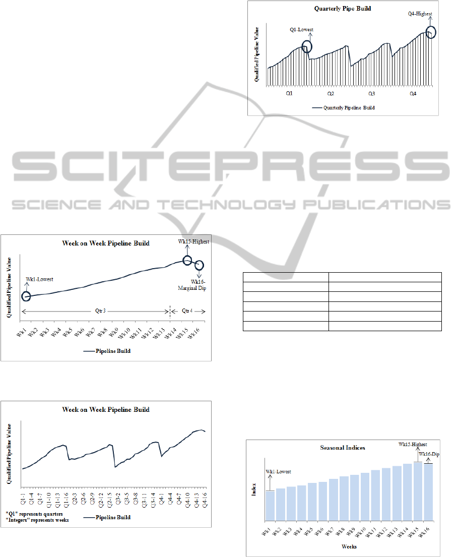
A unique feature of this time series data,
however, is that it has two types of seasonality. The
first type of seasonality is what is observed within
every quarter. The seasonality is across weeks, with
week1 always having the least pipe build, week15
the highest with a marginal dip in week16. It is
during the first two weeks of any quarter (wk14 &
15) that the sales reps concentrate on closing the
deals for the previous quarter and updating them in
the pipeline management tool. For eg: the cleanest
form of pipe available for Q4 is during the third
week of Q4 which is wk16 of the prior quarter. As
shown in figure 2 Weeks 1 to 13 is Q3 and 14 to 16
is the first three weeks of Q4. Post wk16 the
opportunities start closing or moving as it progresses
through the different stages in the sales cycle.
Figure 3: Week on Week pipe build (Illustrative: qualified
pipe values are masked to maintain data privacy).
Figure 4: Pattern observed across one year (Illustrative:
qualified pipe values are masked to maintain data
privacy).
The second type of seasonality is what is observed
across quarters, with Q1 having the least and Q4 the
highest pipe build. This is a pattern that is rampantly
observed in any industry.
Figure 5: Quarterly Seasonality (Illustrative: qualified pipe
values are masked to maintain data privacy).
4.3.1 Data Preparation
Weekly data for 96 weeks was available (08/2009 to
01/2011) for modeling. The data was divided into
development and validation sample. Data for 80
weeks was used to develop the model and data for
16 weeks was used as validation set. The general
statistics of the dataset is as given below:
Table 3: General Statistics of the Sample.
No: of obsevations 96
Mean $623
Standard Deviation $176
Minimum $238
Maximum $1035
Median $625
4.3.2 Deseasonalizing the Data
It was decided to deseasonalize the data with respect
to the weekly seasonality, as the weekly seasonality
was more prominent than the quarterly seasonality.
The quarterly seasonality was to be treated
separately. Seasonality indices were computed using
a 16-point moving average.
Figure 6: Weekly Seasonality (Illustrative: Seasonal
indices are masked to maintain data privacy).
SALES PIPELINE PREDICTION - Predicting a Pipeline using Time Series and Dummy Variable Regression Models
117
The computed seasonal indices showed the weekly
seasonality with week1 being the lowest, week 15
the highest and a marginal dip in week16.
4.3.3 Developing the Trend Line With
Quarterly Seasonality
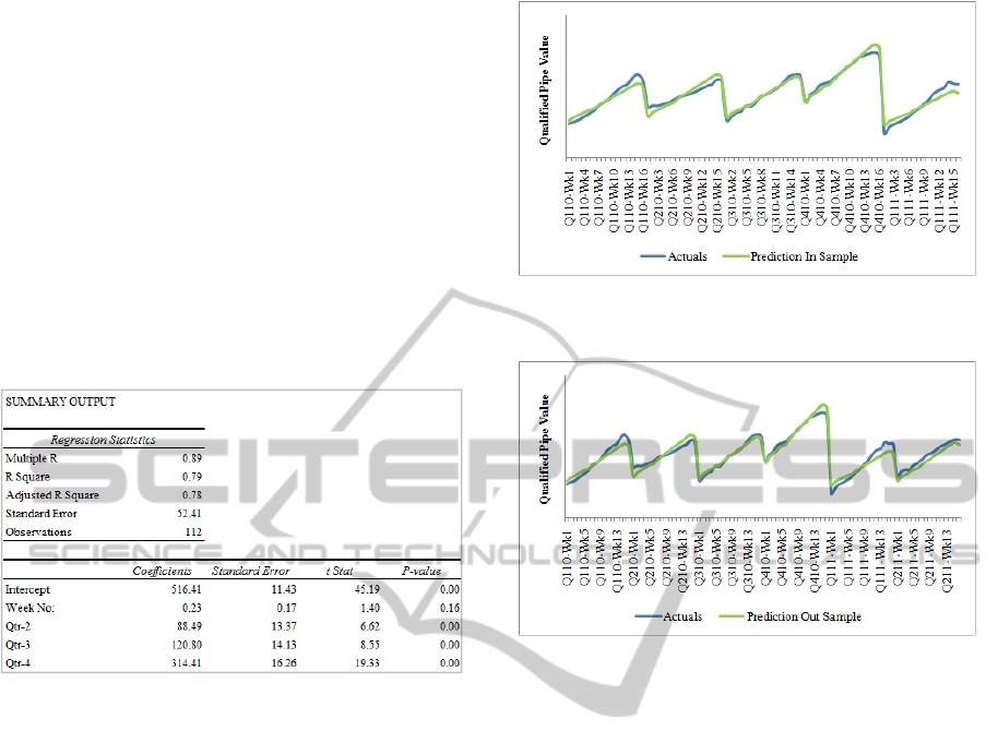
The deseasonalized values were regressed on the
Sales Pipeline to develop the trend line. Dummy
variables were included in the model to capture the
effect of the quarterly seasonality.
The model was found to be significant at α=
0.05. Adjusted R-square of the model is 0.78. Only
Q2, Q3 and Q4 came out as having significant effect
on the prediction.
Figure 7: Result of Regression.
The equation developed to predict sales pipeline
(SP) qualified value is:
(3)
The fourth quarter was found to have the highest
positive impact on the pipeline value
The final prediction with seasonality is derived
by multiplying the predicted pipeline value with the
corresponding seasonality index.
(4)
4.3.4 Model Validation
Sales pipeline value was predicted using the model
and then compared with the actual pipeline value.
Both in sample and out sample validation was done
and the MAPEs (Mean Absolute Percentage Error)
were found to be 6% and 8% respectively. But,
while examining the prediction plots, it was
observed that the model was effectively capturing
the seasonality components (Weekly & Quarterly) as
well as the trend, but it was failing to predict the
sales pipeline at the beginning of every 16-week
cycle accurately.
Figure 8: In Sample Validation (Qualified pipe values are
masked to maintain data privacy).
Figure 9: Out Sample Validation (Qualified pipe values
are masked to maintain data privacy).
It can be observed that if the starting point of every
quarter can be corrected, the trend and volumes
predicted thereafter would match with the actuals.
4.3.5 Triangulation
The fact that the model is not stable at the beginning
of every 16-week cycle can be attributed to the
fluctuations in the first three weeks which is caused
by rep behaviour. To accurately model the starting
point of every quarter extraneous factors such as
market conditions and sales rep motivations will
have to be introduced. Due to lack of data it was
decided not to pursue those efforts.
Instead, a triangulation method was adopted. One
of the best practices in sales pipeline prediction is to
triangulate between historical trends, market vectors
and sales pipeline (Lewis, 2009). The pipeline is
observed during the high flux period (Wk1 to Wk3)
and the prediction is adjusted against the Wk3
actual. By doing so, the MAPE improved to 1%.
5 MODEL DEPLOYMENT
The model was deployed in business successfully.
= 516.4 + 0.23 ∗ + 88.5 ∗
2
+ 120.8 ∗
3
+ 314.4∗
4
(. )
,
=
∗ .
ICORES 2012 - 1st International Conference on Operations Research and Enterprise Systems
118

On testing the results over last two quarters the
pipeline build predicted was less than 0.5% from
actuals. The model was built to drill down to
specific regions and sub regions enabling business to
identify low growth regions in advance and take
corrective measures. Using the historic conversion
rate we are able to derive the likely revenue endpoint
with >98% accuracy.
Figure 10: Prediction Model reporting Schema.
Historical data for the past 92 weeks were
collated and structured into a master database which
acts as the back end to the model. Data cubes by
region/sub region and business units were created in
the data mart. On changing the filters corresponding
values are fed to the report engine and is send for
processing to the prediction engine. Seasonal indices
are recalculated for the new data and the
deseasonalized values are populated. The
deseasonalized values are regressed with the quarter
dummy variables to arrive at the final prediction for
the selected criteria. This data is fed back to the
report engine to provide the final output for the
selected criteria. The model is refreshed every week
with the actuals and irregularities are evened out by
triangulation to the model. The model is used as a
early warning system
6 CONCLUSIONS
The process most often used by sales managers and
companies today is taking a fixed percentage to last
year’s values and then increasing or decreasing the
figure based on the manager’s gut feel to derive the
prediction. Such a technique does not do justice to
the prediction process. While predicting, it is very
important to use a combination of historic data,
statistical modelling and also an in-depth knowledge
of the business.
In this paper, we have demonstrated a
methodology which combines a prediction technique
with business insights to arrive at prediction of sales
pipeline. The model has a prediction accuracy of
99.5%. It provides multiple views, at region, sub-
region and business unit levels, enabling business to
identify low growth areas ahead of time. Corrective
measures can be taken based on these insights.
However, the model is a pure time series model
and not a causal model. This does not take into
account actionable levers like the macroeconomic
factors or sales representative bias and is not capable
of suggesting levers to influence the sales pipeline. It
is restrictive in that respect. Any future research
should be concentrated on building such causal
models.
REFERENCES
Tom, Snyder. 2006. White Paper, Rational Forecasting.
Martin, Lewis. 2009. Webinar, Principal, 3g Selling.
Gilmore, Lewis. 2006. White Paper, How To Develop An
Effective Sales Forecast.
SALES PIPELINE PREDICTION - Predicting a Pipeline using Time Series and Dummy Variable Regression Models
119
