
MULTILEVEL UNIT COMMITMENT IN SMART GRIDS
Maurice G. C. Bosman, Albert Molderink, Vincent Bakker, Gerard Smit and Johann L. Hurink
Dept. of Electrical Engineering, Mathematics and Computer Science, University of Twente, Enschede, The Netherlands
Keywords:
Unit commitment, Smart grids, Column generation.
Abstract:
This paper focuses on the planning of electricity resources in the developing electricity infrastructure. First we
model the existing infrastructure and extend this model to a smart grid infrastructure, where we focus on the
large scale introduction of small electricity generators, leading to generation possibilities at both ends of the
electricity network. Then the traditional Unit Commitment Problem (UCP) is given. We extend this formu-
lation to the Multilevel Unit Commitment Problem (MUCP), where we describe and include the possibilities
that arise in the developing smart grid, in a general way. Based on the characteristics of the problem with its
subdivision into different levels, a planning method for the MUCP is described. Finally we solve and analyze
a scenario, where a fleet of 5000 houses is added to a small collection of power plants.
1 INTRODUCTION
The Unit Commitment Problem (UCP) (Sheble and
Fahd, 1994; Padhy, 2004) is the general term for a de-
cision problem that is related to energy generation. In
this problem, deterministic or stochastic energy de-
mand has to be supplied by a number of generators.
The UCP treats the commitment of specific genera-
tors during certain time windows (i.e. generators are
used to supply (part of) the demand or not) and deter-
mines the generation level of the committed genera-
tors in these time windows.
Traditionally the UCP origins from the situa-
tion where the demand is given as (deterministic or
stochastic) input (Kerr et al., 1966; Groewe-Kuska
and Roemisch, 2005). In the developing smart grid,
new technologies emerge in generation, storage and
consumption (see e.g. (United States Department of
Energy, 2003; Wemhoff and Frank, 2010; Alanne and
Saari, 2004; Lanzafame and Messina, 2010; Ayompe
et al., 2010; Arsie et al., 2009)). This leads to inter-
esting possibilities in demand side load management
and a change in the setting of the UCP. On the one
side, demand side load management gives possibili-
ties to shift demand, such that demand becomes part
of the decision making process rather than being used
as input data. On the other side, different types of
generation with their own characteristics are added to
the set of generators. Many small-sized generators are
distributed over the grid, which leads to a significant
increase in the number of generators that are conside-
red in the UCP.
These advances in the energy supply chain lead to
a new formulation of the UCP, which we call the Mul-
tilevel Unit Commitment Problem (MUCP). Based on
the different sizes and locations in the infrastructure,
a multilevel element is added, taking into account
the quantitative impact of different generators or load
management. To solve this MUCP, the energy infras-
tructure is modeled and partitioned into various lev-
els. The MUCP is part of a three step control method-
ology for smart grids ((Molderink, 2011)) in which
the complete picture of the smart grid is captured: the
methodology consists of prediction, planning and re-
altime control.
The paper is organized as follows. In the next sec-
tion an overview of the energy infrastructure is given
and a model is presented for this structure. Then the
MUCP is formalized in Section 3. In Section 4 the
outlay of a planning method is sketched. As an exam-
ple, a comparison is made between a classic UCP and
the MUCP in Section 5. The results for this compari-
son are analyzed and discussed in Section 6.
2 THE ENERGY
INFRASTRUCTURE
In this section we model the energy infrastructure as a
flow network. First the elements of the electricity grid
are introduced using a small example. Then the grid
is modeled using different elements for production,
361
G. C. Bosman M., Molderink A., Bakker V., Smit G. and L. Hurink J..
MULTILEVEL UNIT COMMITMENT IN SMART GRIDS.
DOI: 10.5220/0003716903610370
In Proceedings of the 1st International Conference on Operations Research and Enterprise Systems (ICORES-2012), pages 361-370
ISBN: 978-989-8425-97-3
Copyright
c
2012 SCITEPRESS (Science and Technology Publications, Lda.)
consumption, transportation and communication.
The classic energy infrastructure (or supply chain)
can be clearly separated into a consumption and a pro-
duction side. Consumption of energy (gas, electricity,
heat, etcetera) can be predicted quite accurately, based
on historic demand and currently available charac-
teristics (of consumer behaviour, weather, etcetera)
(Bakker et al., 2010). In this classic situation, the
energy production of power plants is completely ad-
justed to match this demand. Through transmission
and distribution networks this production is brought
to the consumer. In Figure 1 a simplified example of
a
b
c
d
e
f
g
h
i
x
a
|7
x
b
|8
x
c
|5
8|20
2|5
1|5
2|5
3|5
Figure 1: An example of the classic electricity infrastruc-
ture.
the situation in a certain time period is given, in which
a decision has to be made on the generation output of
three generators a, b and c, where demand is located
in f, g, h and i. The directed edges (e, f), (e, g), (e, h)
and (e, i) represent the distribution network. The ca-
bles in this part of the network have a certain demand
from the end points (e.g. villages, industrial areas)
and a fixed network capacity for the given time pe-
riod, which are given as weights demand|capacity.
The aggregated demand of the end points f, g, h and i
has to be supplied by the transmission network, which
is represented by the directed edge (d, e). This de-
mand eventually has to be produced by the three gen-
erators, which have a different production capacity. In
this case, all demand can be supplied by generator b
alone, whereas a combination of generators has to be
committed when a or c is willing to produce, since
their production capacity is insufficient to supply the
actual demand alone.
In the current flow network of the example, there
is no bottleneck. Even if all end points would ask
maximum demand (i.e. a demand equal to the distri-
bution grid capacity), the transmission grid is able to
supply this amount of electricity, and the three gener-
ators can produce this amount. When the classic in-
frastructure changes into the new smart grid, the clas-
sic division into a production and a consumption side
becomes less clear. The original consumers also have
the possibility to produce, which results in a bidirec-
tional network. This might put more stress on the ex-
isting infrastructure. In this paper we assume that the
transmission/distribution capacity of the correspond-
ing networks is sufficient even for extreme demands.
village
village
village
village
MV grid
transformer
HV grid
power plant
power plant
power plant
Figure 2: A model of the classic electricity infrastructure.
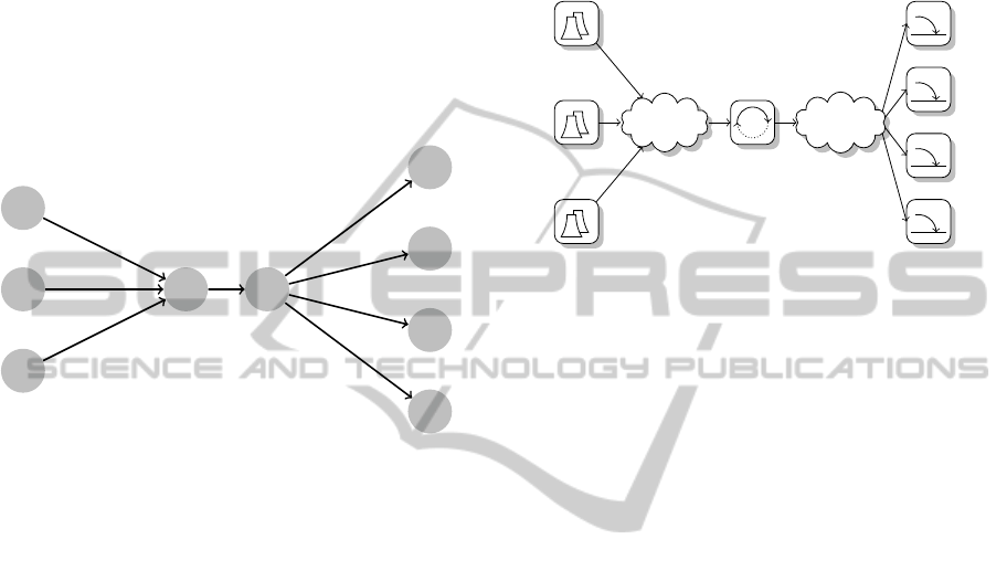
In Figure 2 the classic infrastructure of Figure 1
is modeled again, by using different types of nodes
to stress the differences between generation, trans-
portation and consumption. This model allows to
model flows of different types, with preservation of
energy, as proposed by (Molderink, 2011). As indi-
cated in this model, we introduce additional nodes
compared to Figure 1, drawn as clouds, which rep-
resent the level of the grid. The power plants are con-
nected to the high voltage grid, which is connected
to the medium voltage grid, via a transformer. The
demand of the example is connected to this medium
voltage grid. In the Unit Commitment Problem, the
following challenge for the power plants has a cen-
tral position: how to supply the given demand by
the available generation possibilities, such that the
total generation is done under minimum operational
costs? Operational costs can be divided into energy
(fuel efficiency) and cost effective costs (maintenance
and startup/shutdown costs) (Sheble and Fahd, 1994;
Padhy, 2004).
Figure 3 shows the extended infrastructure. As
in Figure 2, directed edges show the electricity flow
in the network. Some edges are bidirectional, in-
dicating that a flow in both ways is possible. The
large power plants are connected to the high voltage
grid; smaller generation (e.g. windmill/solar panel
parks, biogas installations, etcetera) is connected to
the medium voltage grid. Note that this smaller gen-
eration is not directly coupled to the medium voltage
grid, but via an additional electricity node, which is
connected to an exchanging node, called ‘new gen-
eration’. This ‘exchanger’ expresses the introduction
of a new, lower level in the model of the smart grid
ICORES 2012 - 1st International Conference on Operations Research and Enterprise Systems
362

village
house
MV grid
transformer
HV grid
power plant
power plant
power plant
village
village
village
transformer
LV grid
village
electr.
house house house
electr.
local consumption
microCHP
gas
gas
gas network
heat loss
heat buffer loss
heat
heat demand
new generation
windmill
solar panels biogas
electr.
Figure 3: A model of the smart grid infrastructure.
and functions as a separator between the optimization
problem on the higher level and the local commitment
problem on the lower level (e.g. the smaller genera-
tion). The exchanger can be seen as a communication
means between higher and lower order planning prob-
lems. This division into levels is further explained in
Section 4.
Compared to the model of Figure 2, areas like vil-
lages are now modeled in more detail. In the previ-
ous model it sufficed to consider the connection of a
village to the medium voltage grid, since only aggre-
gated demand is taken into account. In the extended
model a village is connected to the lower voltage grid
and an exchanger is used to specify a lower level.
In this lower level, a next level is introduced for the
houses to model their own generation/consumption
characteristics. Within the model (e.g. within the
houses) different types of energy (i.e. gas and heat)
are combined. This is one of the strengths of the ex-
tended model. In the model presented in Figure 3 we
show the modeling of a microCHP (Combined Heat
and Power generation on a household level (United
States Department of Energy, 2003)), which is a de-
vice that consumes natural gas and produces both heat
and electricity at a fixed ratio. It is convenient to use
a heat buffer next to this microCHP to guarantee the
heat supply in the house and to partially decouple heat
consumption from the generation of heat (and elec-
tricity). In the model, gas import information is stored
in the gas exchanger. The energy efficiency of gener-
ation can be modeled by adding energy losses. In the
example, the loss flow of the microCHP has a fixed ra-
tio to the heat and electricity generation; the loss flow
of the heat buffer is determined by the state of the
buffer. In a similar way, the efficiency of each type
of generation can be modeled. However, for simplic-
ity this is left out of Figure 3 and we do not consider
efficiency in the remainder of this paper.
3 THE MULTILEVEL UNIT
COMMITMENT PROBLEM
This section describes the Multilevel Unit Commit-
ment Problem. Starting from the Unit Commitment
Problem we derive additional constraints to formulate
the MUCP.
The classic UCP aims to minimize operational
costs or to maximize the profit of the system of gener-
ators. We consider the problem of minimizing costs.
Operational costs are depending both on the binary
commitment variables u
i, j
(specifying whether gener-
ator i is committed or not in time period j) and on the
production level x
i, j
(specifying the electricity pro-
duction of generator i in time period j). In general
the operational costs can be described by a function
f(u, x), where the variables u and x run over the time
horizon T for N generators. Note that startup costs
are incorporated in this notation. The objective of the
UCP is then to minimize f(u, x). Some common con-
straints that are mostly used in the UCP are given in
formulation (1)-(9).
MULTILEVEL UNIT COMMITMENT IN SMART GRIDS
363

min f(u, x) (1)
s.t.
∑
i
x
i, j
≥ d
j
∀ j (2)
∑
i
(u
i, j
x
max
i
− x
i, j
) ≥ r
j
∀ j (3)
u
i, j
x
min
i
≤ x
i, j
≤ u
i, j
x
max
i
∀i, j (4)
s
down
i
≤ x
i, j
− x
i, j−1
≤ s
up
i
∀i, j (5)
u
i, j
≥ u
i, j−k
− u
i, j−k−1
∀i, j, k = 1, . . . , t
mr
i
− 1 (6)
1− u
i, j
≥ u
i, j−k−1
− u
i, j−k
∀i, j, k = 1, . . . , t
mo
i
− 1 (7)
u
i, j
∈ {0, 1} ∀i, j (8)
x
i, j
∈ R
+
∀i, j (9)
Equation (2) requires that the total production sat-
isfies the total demand; equation (3) asks for a cer-
tain amount of spinning reserve r
j
, i.e. the additional
available generation capacity of already committed
generators. This constraint is added to guarantee a
certain amount of flexibility in the case of a higher-
than-predicted demand or in the case of a failure of a
certain generator. The production boundaries of the
generators x
min
i
and x
max
i
are defined in equation (4)
and the ramp up and ramp down rates s
up
i
and s
down
i
,
which determine the speed with which generation can
be adjusted, are given in equation (5). Equations (6)
and (7) state that the generator has to stay up and run-
ning (or stay switched off) once a corresponding deci-
sion to switch it on (or off) has been made within the
last t
mr
i
(t
mo
i
) time periods. The decisions to commit a
generator are binary decisions, where the production
decisions are real numbers.
When we consider the developing energy infras-
tructure, we see more decentralized energy produc-
tion y
m, j
, where y
m, j
specifies the electricity produc-
tion of local generator m in time period j. The maxi-
mum production of these types of generators is much
smaller than the minimum production of a power
plant: max
m
(y
max
m
) ≪ min
i
x
min
i
. However, there
may be very many of them. The local generators
are often more limited in their production decisions
than normal power plants, especially when we con-
sider combined heat and electricity generation (e.g.
micro/mini Combined Heat and Power). In this case
the heat demand of the local household/glasshouse
determines to a large extent the total daily generation,
where some flexibility is provided by the use of a heat
buffer. Also, the power output is completely deter-
mined for many of these generators, once the gener-
ator is in operational mode. This further limits the
flexibility of the decision maker.
In the developing energy infrastructure, also a lot
of renewable generation is introduced, which more
and more takes place on a local scale. To cope with
these changes we extend the given UCP formulation
in the following way to a MUCP formulation.
min f(u, x)− g(p, u, y) (10)
s.t.
∑
i
x
i, j
+
∑
m
y
m, j
≥ h
j
(d) ∀ j (11)
∑
i
(u
i, j
x
max
i
− x
i, j
) ≥ r
j
∀ j (12)
z
min
j,F
n
≤
∑
m∈F
n
j
∑
k=1
y
m,k
≤ z
max
j,F
n
∀ j, n (13)
u
i, j
x
min
i
≤ x
i, j
≤ u
i, j
x
max
i
∀i, j (14)
s
down
i
≤ x
i, j
− x
i, j−1
≤ s
up
i
∀i, j (15)
u
i, j
≥ u
i, j−k
− u
i, j−k−1
∀i, j, k = 1, . . . , t
mr
i
− 1 (16)
1− u
i, j
≥ u
i, j−k−1
− u
i, j−k
∀i, j, k = 1, . . . , t
mo
i
− 1 (17)
u
m, j
≥ u
m, j−k
− u
m, j−k−1
∀m, j, k = 1, . . . , t
mr
m
− 1 (18)
1− u
m, j
≥ u
m, j−k−1
− u
m, j−k
∀m, j, k = 1, . . . , t
mo
m
− 1 (19)
y
min
m, j
≤
j
∑
k=1
y
m,k
≤ y
max
m, j
∀m, j (20)
y
m, j
= l(u
m
) ∀m, j (21)
u
i, j
, u
m, j
∈ {0, 1} ∀i, m, j (22)
x
i, j
, y
m, j
∈ R
+
∀i, m, j (23)
The formulation of the MUCP is given by equations
(10)-(23), where the original UCP can be found in
equations (11),(12) and (14)-(17). In this MUCP
model we also incorporate demand side load manage-
ment to alter the demand. This is formalized in equa-
tion (11) by the function h
j
(d). Furthermore, the lo-
cal generation y
m, j
is taken into account in this equa-
tion too. The local generators have the same type of
dependency constraints on runtime and offtime over
time periods (equations (18) and (19)) as the large
generators (equations (16) and (17)). Next to these
machine dependency constraints the generators also
have user dependencies, resulting e.g. from the heat
demand. The use of a heat buffer, with some ini-
tial heat level, in combination with the local heat de-
mand, determines the minimum aggregated heat pro-
duction and the maximum aggregated heat produc-
tion. Since heat and electricity production are directly
coupled, we model this relationship using a minimally
required aggregated electricity production y
min
m, j
and a
maximally allowed aggregated electricity production
y
max
m, j
, as in equation (20). So, possible decisions in
future intervals are not only influenced directly via
runtime/offtime constraints, but they are also influ-
enced indirectly via equation (20). As stated before,
the generator output is completely determined by the
commitment decisions, as in equation (21).
The planning problem for only a group of mi-
croCHPs is proven to be NP-complete in the strong
sense, due to the two-dimensional aspect of the prob-
lem (i.e. a strong dependency between generation in
time periods and a strong dependencybetween house-
holds due to the aggregated generation in the fleet)
ICORES 2012 - 1st International Conference on Operations Research and Enterprise Systems
364

(Bosman et al., 2010). It is therefore practically in-
tractable to solve the MUCP (of which the planning
problem for a fleet of microCHPs is only a part of
the problem) directly. However, heuristics have been
developed to solve the planning problem for the fleet
(Bosman et al., 2011). For this reason, a planning
method for the MUCP is presented that uses the natu-
ral division into different production levels to separate
the decisions that haveto be made for the power plants
and for the local generators, and still combine the two
into a global Multilevel Unit Commitment decision
problem.
In the MUCP, a group of local generators (called
a fleet) is considered as one entity on the planning
level, equivalent to a power plant. Of course, a sub-
division in multiple entities F
n
is allowed. Equation
(13) is applied to these n fleets, which forces the ag-
gregated production of all generators to be within up-
per and lower bounds z
max
j,F
n
and z
min
j,F
n
. The most natu-
ral bounds are z
max
j,F
n
=
∑
m∈F
n
y
max
m, j
and z
min
j,F
n
=
∑
m∈F
n
y
min
m, j
.
These bounds may be sharpened further, since not all
possible decision paths (sequences) within these nat-
ural bounds may be feasible. We explain this by giv-
ing two examples. As a first example, the capacity of
the fleet may be smaller than
∑
m∈F
n
y
max
m, j
−
∑
m∈F
n
y
min
m, j−1
,
which may result in a fleet decision in time period j
that cannot be met by the individual generators. This
would require additional bounds on the production ca-
pacity of the fleet entity.
However, even if the fleet decision respects the ca-
pacity of the fleet and if the fleet decision path stays
within the natural bounds
∑
m∈F
n
y
max
m, j
and
∑
m∈F
n
y
min
m, j
, it
can be impossible to follow this decision path by the
individual generation, as shown in the second exam-
ple by Figure 4. Figure 4(a) and 4(b) show the possi-
ble decision paths within the natural bounds (the gray
area) for two households equipped with a microCHP;
Figure 4(c) shows the combined decisions, includ-
ing capacity constraints, for which the given decision
path in Figure 4(d) is impossible to follow. Although
the two generators may run simultaneously, indepen-
dently in the fourth or in the fifth time period, it is
impossible to have the two generators running simul-
taneously in these time periods subsequently, due to
the limited possibilities for the second household in
the fourth and fifth time periods. So, even when ca-
pacity constraints are added the natural bounds may
not result in a fleet entity decision that is feasible for
the individual generators. This is the reason why the
natural bounds may be sharpened. Also, to guarantee
stability, especially within the distribution network,
additional constraints may be posted to the output of
time
total production
(a) Possible transitions of one microCHP.
time
total production
(b) Possible transitions of another microCHP.
time
total production
(c) Addition of feasible regions and possible transi-
tions of the combination.
time
total production
(d) Construction of a bid pattern which is impossible
to follow.
Figure 4: A counterexample for the natural fleet bounds.
MULTILEVEL UNIT COMMITMENT IN SMART GRIDS
365

fleets of small generators.
Since the operation of the individual small gener-
ators is of minor importance in comparison with the
behaviour of the fleet, we do not wish to minimize op-
erational costs for the fleet(s). In the additional func-
tion g(p, u, y) in equation (10) the profit of the fleet is
maximized, when this fleet operates, using the given
bounds, on an electricity market with prices p
j
.
4 A PLANNING METHOD FOR
THE MUCP
In Section 2 the smart grid is modeled using a divi-
sion into different levels. This division is based on
the amount of energy the different generators produce
and forms the base for a leveled approach to solve the
MUCP of Section 3. In this section, a sketch of a plan-
ning method is given, introducing patterns as building
blocks for the method.
Since it is practically intractable to combine the
commitment of large and small types of generation,
information on the smaller generation is aggregated
on a higher level by using the exchangers, as shown in
the previous sections. Each fleet (e.g. village, wind-
mill park) is then considered as one entity, with some
global constraints based on the aggregated informa-
tion, and treated in this simplified form in the opti-
mization problem. Note that on this high level, local
constraints on the smaller generators are discarded in
the optimization problem. The objective function of
this high level optimization problem reflects the orig-
inal objectives; operational costs are minimized for
power plants and the common fleet output is maxi-
mized for its profit on an electricity market. The deci-
sion paths that result from the optimization of the high
level optimization problem for all entities (whether
power plants or fleets) are called patterns. For a power
plant this pattern simply reflects the commitment (and
generation level) decisions that have to be made; for
a fleet this pattern is the input for a new, lower level
optimization problem.
On the lower level a new optimization problem is
formed, which is to match the provided fleet pattern
with the available individual generation possibilities
as good as possible. So, the objective is to minimize
the deviation from the (higher level) fleet pattern. A
fleet consisting of small generators can sometimes be
optimized using full knowledge about each genera-
tor (i.e. patterns can be derived directly for biogas
installations, windmill parks, etcetera, based on lo-
cal constraints on these types of generation). How-
ever, for a fleet consisting of houses it is harder to
solve an overall optimization problem in reasonable
time, where the full details of all houses are consid-
ered, especially when the number of houses is large.
In this situation, a next level is introduced, using a
column generation approach to provide the fleet opti-
mization problem with so-called house patterns. The
lower level optimization problem has to select indi-
vidual house patterns in order to allow the fleet plan-
ner to find a combination of patterns that minimizes
the deviation from the fleet pattern. Based on infor-
mation from the solution of the higher level optimiza-
tion problem, a column generation technique is used
to extend the current pattern set for each house with
new promising patterns.
Once the fleet patterns are locally optimized, the
resulting patterns of the fleet planning problem that
minimize the deviation from the original fleet pat-
terns, are now communicated back to the high level
optimization problem. Using this information, this
problem is solved again. This can be seen as a clas-
sic UCP with altered demand (and possibly altered
spinning reserve). If the result is not satisfying, addi-
tional constraints on the fleet patterns can be added to
the original high level optimization problem, and the
complete process can be repeated.
5 CASE STUDY
To study the influence of generation on multiple lev-
els in the electricity grid, we set up a scenario with
two levels. We choose to use two levels, to see the in-
teraction between generators of different production
capacity in a direct way. In this illustrative example
we use 10 generators on the highest level, with a to-
tal production capacity of 15 MW. This capacity is
divided over 5 generators with a capacity of 1 MW
and a minimum production level of 0.5 MW, and 5
generators with a capacity of 2 MW and a minimum
production level of 1 MW. The (absolute) ramp up
and ramp down rates are equal to the minimum pro-
duction for each power plant. Between the maximum
and minimum production values the operator of the
generator has flexibility to choose its power output,
once the unit is committed. The minimum runtime
and offtime are set to half an hour.
On the lowest level, we have 5000 houses con-
taining a generator, with a total capacity of 5 MW.
These generators are microCHPs (Combined Heat
and Power systems on a household scale) with a pro-
duction output of 1 kW. This power output is a direct
result from the decision to run the microCHP on a
certain moment in time. This means that there is no
flexibility in the production level of committed units,
although flexibility can be found in the moments in
ICORES 2012 - 1st International Conference on Operations Research and Enterprise Systems
366
time that the units are committed. However, these mo-
ments are further constrained by the heat demand in
the houses: the maximum production of the fleet over
the planning horizon is 39.8 MWh and the minimum
production is 35.1 MWh, which is of the same order
of committing a power plant for a complete day. The
minimum runtime and offtime are again set to half an
hour.
In the scenario we define four use cases to study
the influence of introducing a fleet of microCHPs in
the UCP. For each use case we use time periods of
30 minutes length; the commitment is planned for a
complete day, which comes down to 48 time periods.
The total daily demand is 114.2 MWh, with a peak of
8 MW and a base load of 2.5 MW. In this scenario
we do not consider demand side load management.
We require a spinning reserve of 2 MW at all time
periods. The objective function combines operational
costs for the power plants and profit maximization for
the fleet. The first use case is based on real prices
from the APX day ahead market
1
. In the second use
case we multiply all prices with −1, which creates
artificial negative values, to compare to what extent
the fleet would change its decisions. The third use
case uses artificial prices that correspond to the daily
electricity demand; the higher the demand, the higher
the price. This use case is defined to verify if the fleet
can behave in such a way that peak demand can be
decreased and the demand for the power plants can
be flattened. The fourth use case is the opposite of the
third case, in the sense that prices are again multiplied
with −1; the higher the demand, the lower the price.
0 200 400
600
800 1,000
0
1,000
2,000
3,000
4,000
generation per 30 minutes (kWh)
costs
power plant 1|3|5 power plant 2|4
power plant 6|8|10 power plant 7|9
Figure 5: The operational cost functions of the power
plants.
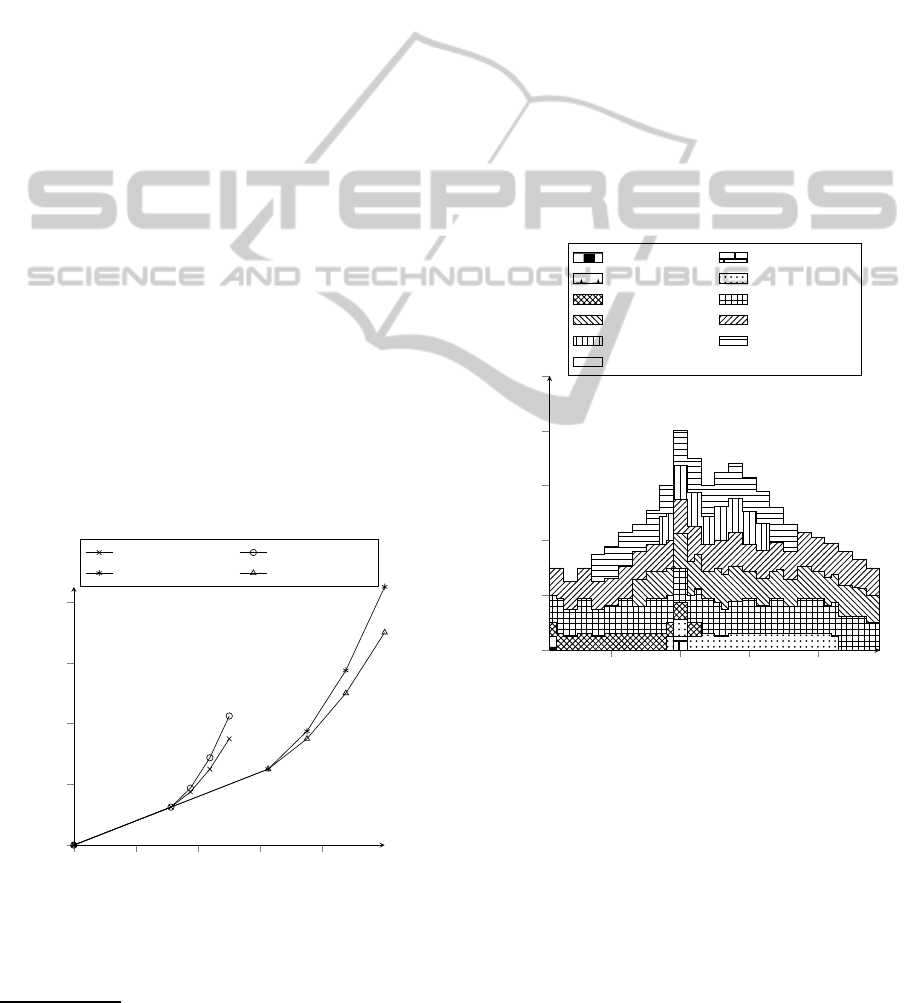
In Figure 5 the cost functions of the power plants
1
http://www.apxendex.com
are given. They are modeled as piecewise linear cost
functions, to approximate quadratic operational cost
functions. Below certain production levels (625 kWh
for the large power plants and 312.5 kWh for the
small power plants) the cost functions are equal, and
power plants are mutually exchangeable. The start of
a power plant is furthermore penalized with a cost of
1000.
The different optimization problems are mod-
eled as Integer Linear Programming formulations in
AIMMS modeling software using CPLEX 12.2 as
solver. The solution method is executed on a desk-
top computer (2.40 GHz and 2.00 GB RAM).
6 RESULTS AND DISCUSSION
In this section we discuss the solutions of the four use
cases, which are found by the planning method.
10 20 30 40
0
1,000
2,000
3,000
4,000
5,000
30 minutes intervals
generation (kWh)
power plant 1 power plant 2
power plant 3 power plant 4
power plant 5 power plant 6
power plant 7 power plant 8
power plant 9 power plant 10
local generation
Figure 6: The solution of the UCP.
Figure 6 shows the detailed solution of the UCP,
where we do not use the 5000 houses and the de-
mand is fullfilled against minimal operational costs.
The commitment and corresponding generation pat-
terns are given for the 10 power plants. This solution
is used to validate the optimization model. At any
time period, the spinning reserve of 1000 kWh (=2
MW for time periods of 30 minutes length) is avail-
able within this solution. The ramp rates are taken
into account; the minimum and maximum production
constraints are considered too. This can best be seen
when a generator shuts down. The time period before
MULTILEVEL UNIT COMMITMENT IN SMART GRIDS
367

a generator shuts down, the production is reduced to
the minimum production level, which happens to be
equal to the (absolute) maximum ramp up and ramp
down rates. In this case the generator may shut down
in the next period. We see that nine of the ten units are
committed during the day; each power plant is started
at most once.
Table 1 shows the results for the MUCP, where
we incorporate the fleet of 5000 houses. The table
shows the operational costs of the power plants, both
for the initial planning with the rough fleet constraints
(rough) and for the final result after applying the col-
umn generation to the fleet and replanning the power
plants using the elaborated fleet pattern (result). It
also shows the number of starts for the power plants,
again for the rough planning and for the final re-
sult. The computational time of the result includes the
computational time of the rough planning. Regard-
ing the fleet planning, the final mismatch to the rough
planning (i.e. absolute deviation from the rough plan-
ning) is given in kWh and in percentage of the total
generation of the rough planning. The resulting total
generation is given in the last row of Table 1. Since
we mostly use artificial prices for the electricity mar-
ket, we do not show the profit maximization of the
fleet in more detail.
The operational costs of the result are relatively
close to the rough planning operational costs in all
cases. This means that the commitment of the power
plants is not altered too drastically after the elaborated
planning of the fleet; so, the planning method be-
havesas expected. Of course the final costs are higher,
since the rough planning gives the optimal combina-
tion of power plant operation and fleet operation. The
four use cases show that we are able to steer the fleet
production by using different prices. The number of
starts of the power plants increases in all cases, ex-
cept for the third use case. In case 3 the power plants
need only 5 starts in the final fleet planning. This
is mostly due to the initial fleet planning, which is
aimed to reduce the peaks in the demand. In the re-
alization of this planning the fleet has relatively much
difficulties, since the mismatch from the rough plan-
ning is the highest of the four cases. Nevertheless this
realization leaves enough possibilities for the power
plants to find a planning that only needs 5 commit-
ments. The big advantage is that the fleet does not
interfere too much with the base load, which simpli-
fies the continuity of the commitment in time periods
with low demand.
The computational time of the planning method
stays below half an hour in all cases. This is accept-
able for a practical application, especially since the
column generation technique can be distributed over
the smart grid in real life. The mismatch from the
rough planning is below 8%. Figure 7 shows the de-
0 2 4
6
8 10 12
0
0.2
0.4
0.6
0.8
1
1.2
·10
4
iterations
total mismatch (kWh)
case 1 case 2
case 3 case 4
Figure 7: The mismatch during the column generation for
the four use cases.
velopment of the mismatch during the column genera-
tion method. The final solution is found after approxi-
mately 10 iterations. The existence of a mismatch can
be partly explained by a possible impractible rough
planning, but also by the fact that we used a maxi-
mum runtime of 60 seconds for the pattern matching
problem, which tries to select exacly one pattern for
each house to minimize the mismatch from the rough
planning. This maximum runtime results in a prelimi-
nary abortion of the solution method in all four cases.
From this we may conclude that the fleet might have
done better, to the costs of higher computational time.
Finally we see that the total fleet production approx-
imates the upper production bound of 39.8 MWh in
use cases 1, 3 and 4, whereas the total fleet produc-
tion in case 2 is close to the lower production bound
of 35.1 MWh. This indicates that the prices in case 2
are too negative, such that it is more cost effective to
let the power plants produce more.
Figure 8 shows the unit commitment of the 10
power plants and the fleet production of the 5000
houses in the second use case. Figure 8(a) gives the
rough fleet planning and Figure 8(b) gives the result-
ing, final fleet planning. We show this use case in
more detail to describe two phenomena that occur.
Firstly, we see three short periods of commitment
of the small power plants 1 and 3 in the final plan-
ning. These commitments are not necessary to full-
fill the demand; the already committed power plants
could have supplied this additional demand them-
selves, even against lower costs. However,in that case
ICORES 2012 - 1st International Conference on Operations Research and Enterprise Systems
368
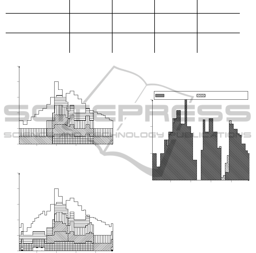
Table 1: MUCP results for the four cases.
case 1 case 2 case 3 case 4
rough detailed rough detailed rough detailed rough detailed
operational costs 158748 164846 163593 169325 154748 163230 154748 167730
# of starts
5 6 5 8 5 5 5 9
computational time (s) 32.28 1543.10 26.91 1798.19 61.72 1753.56 7.40 1451.00
mismatch (kWh) 2236.5 986 3099.5 478.5
mismatch/rough prod. (%)
5.6 2.8 7.8 1.2
fleet production (kWh) 38926 35589 37927 38868.5
10 20 30 40
0
1,000
2,000
3,000
4,000
5,000
30 minutes intervals
generation (kWh)
(a) The solution of the high level MUCP.
10 20 30 40
0
1,000
2,000
3,000
4,000
5,000
30 minutes intervals
generation (kWh)
(b) The solution of the high level MUCP, including a de-
tailed fleet planning.
Figure 8: The second use case in more detail.
there would not be sufficient spinning reserve left in
the committed power plants. For this reason, power
plants 1 and 3 have to be committed during these pe-
riods. Secondly, we see many different generators
committed in the final planning, in comparison with
the rough planning. However, as we have stated be-
fore, below certain production levels (625 kWh for the
large power plants and 312.5 kWh for the small power
plants) the cost functions are equal, and power plants
are mutually exchangeable. This could explain the
larger number of committed generators. Finally, we
10 20 30 40
0
500
1,000
1,500
30 minutes intervals
total generation (kWh)
rough planning final found solution
Figure 9: Comparison of rough planning and final found so-
lution for the planning of the local generators in the second
use case.
show the rough fleet planning and the final fleet plan-
ning in one overview in Figure 9. This figure shows
that the rough planning is matched reasonably well.
6.1 Summary
This paper presents a Multilevel Unit Commitment
Problem (MUCP) for the infrastructure of a smart
grid. This MUCP differs from the common Unit
Commitment Problem (UCP) in its size, the differ-
ence in production levels of the different generator
types, the possibility of demand side load manage-
ment and storage. Objectives may also differ due to
developments in the electricity markets, which leads
to a partial focus shift from the optimization of the
operational costs of generators to the optimization of
the behaviour on the electricity market. In this paper
a use case is defined where a group of 5000 houses
is added to a normal UCP instance, which is planned
MULTILEVEL UNIT COMMITMENT IN SMART GRIDS
369

using the proposed planning method. The results of
the given scenario show that the presented approach
can be applied to a fleet size of 5000 houses.
6.2 Recommendations
In future work scalability should be validated; is it
possible to solve an extended scenario, where multi-
ple fleets are optimized simultaneously? Regarding
this extended scenario, the fleet sizes should be ana-
lyzed for their contribution to the high level optimiza-
tion problem and the speed and quality of the under-
lying lower level optimization problem(s). In this ex-
tended scenario, the influence of the production ca-
pacity of low level generators on the capability to ad-
just the total output as a fleet also has to be studied.
Also demand side load management should be
added, as well as other local generation or storage
technologies, such as solar cells and heat pumps, to
solve an extended real life Multilevel Unit Commit-
ment Problem. Other types of local generation, de-
mand side load management and local storage can
be incorporated in a similar way as is done for the
microCHP. However, these possibilities cannot be
treated as independent fleets. An additional level
needs to be introduced in the MUCP, where the in-
teractions between these possibilities are considered
as a new type of combined patterns.
REFERENCES
Alanne, K. and Saari, A. (2004). Sustainable small-scale
chp technologies for buildings: the basis for multi-
perspective decision-making. Renewable and Sustain-
able Energy Reviews, 8(5):401–431.
Arsie, I., Marano, V., Rizzo, G., and Moran, M. (2009). In-
tegration of wind turbines with compressed air energy
storage. In Proceedings of the Second Global Con-
ference on Power Control and Optimization (PCO),
pages 11–18. Keynote lecture.
Ayompe, L. M., Duffy, A., McCormack, S. J., and Con-
lon, M. (2010). Validated real-time energy models
for small-scale grid-connected pv-systems. Energy,
In Press, Corrected Proof.
Bakker, V., Bosman, M. G. C., Molderink, A., Hurink, J. L.,
and Smit, G. J. M. (2010). Improved heat demand
prediction of individual households. In Proceedings
of the first Conference on Control Methodologies and
Technology for Energy Efficiency, Vilamoura, Portu-
gal, pages 1–6, Oxford. Elsevier Ltd.
Bosman, M. G. C., Bakker, V., Molderink, A., Hurink, J. L.,
and Smit, G. J. M. (2010). On the microchp schedul-
ing problem. In Proceedings of the Third Global Con-
ference on Power Control and Optimization (PCO),
pages 367–374.
Bosman, M. G. C., Bakker, V., Molderink, A., Hurink, J. L.,
and Smit, G. J. M. (2011). Controlling a group of
microchps: planning and realization. In Proceedings
of the First International Conference on Smart Grids,
Green Communications and IT Energy-aware Tech-
nologies (ENERGY 2011), pages 1–6.
Groewe-Kuska, N. and Roemisch, W. (2005). Stochastic
Unit Commitment in Hydrothermal Power Production
Planning. Society for Industrial and Applied Mathe-
matics, Philadephia, PA.
Kerr, R., Scheidt, J., Fontanna, A., and Wiley, J. (1966).
Unit commitment. Power Apparatus and Systems,
IEEE Transactions on, PAS-85(5):417 –421.
Lanzafame, R. and Messina, M. (2010). Power curve con-
trol in micro wind turbine design. Energy, 35(2):556–
561. ECOS 2008, 21st International Conference, on
Efficiency, Cost, Optimization, Simulation and Envi-
ronmental Impact of Energy Systems.
Molderink, A. (2011). On the three-step control method-
ology for Smart Grids. PhD thesis, University of
Twente.
Padhy, N. (2004). Unit commitment-a bibliographical
survey. Power Systems, IEEE Transactions on,
19(2):1196 – 1205.
Sheble, G. and Fahd, G. (1994). Unit commitment litera-
ture synopsis. Power Systems, IEEE Transactions on,
9(1):128 –135.
United States Department of Energy (2003). The micro-
CHP technologies roadmap. Results of the Micro-
CHP Technologies Roadmap Workshop.
Wemhoff, A. and Frank, M. (2010). Predictions of energy
savings in hvac systems by lumped models. Energy
and Buildings, 42(10):1807 – 1814.
ICORES 2012 - 1st International Conference on Operations Research and Enterprise Systems
370
