TOWARDS COGNITIVE STEERING BEHAVIOURS FOR

TWO-WHEELED ROBOTS

Franc¸ois Gaillard

1,2

, C´edric Dinont

, Micha¨el Soulignac

and Philippe Mathieu

ISEN Lille, CS Dept., 41, Boulevard Vauban, 59046 Lille Cedex, France

LIFL, University of Lille 1, UMR USTL/CNRS 8022, 59655 Villeneuve d’Ascq Cedex, France

Keywords:

Robot and multi-robot systems, Cognitive robotics, Task planning and execution, Steering behaviours.

Abstract:

We present a two-layer architecture for two-wheeled robots trajectory planning. This architecture can be used

to describe steering behaviours and to generate candidate trajectories that will be evaluated by a higher-level

layer before choosing which one will be followed. The higher layer uses a TÆMS tree to describe the current

robot goal and its decomposition into alternative steering behaviours. The lower layer uses the DKP trajectory

planner to grow a tree of spline trajectories that respect the kinematic constraints of the problem, such as

linear/angular speed limits or obstacle avoidance. The two layers closely interact, allowing the two trees to

grow simultaneously: the TÆMS tree nodes contain steering parameters used by DKP to generate its branches,

and points reached in DKP tree nodes are used to trigger events that generate new subtrees in the TÆMS tree.

We give two illustrative examples: (1) generation and evaluation of trajectories on a Voronoi-based roadmap

and (2) overtaking behaviour in a road-like environment.

1 INTRODUCTION

Our aim is to provide human-like steering behaviours

to autonomous mobile robots with the respect of their

physical constraints. We would like to design robotic

applications using high-level building blocks repre-

senting motion strategies like follow or overtake and

behaviours like drive smoothly or drive aggressively.

This kind of problem has already been addressed

for autonomous simulated characters by (Reynolds,

1999) who proposed a two-layer architecture to ex-

press steering behaviours.

We reuse here the basic idea from Reynolds but

transposing on real-world robots results that work

for simulating characters raises some problems. The

main one lies in the link between the cognitive layer

of the robot and the trajectory planning layer. An

action selection level ﬁrst decides which high-level

goals are given to the motion planning layer. Such

an approach hides the motion planning and locomo-

tion problems, so the completeness and kinodynamic

constraints respect issues exist. The action selection

level cannot verify the trajectory feasibility of the de-

cisions and it appears difﬁcult to encode the kinody-

namic constraints within this level.

In the context of robotic arms, some recent ad-

vances have been done in mixing planning, using

PDDL for instance (McDermott et al., 1998), and mo-

tion planning when the conﬁguration space can be en-

tirely precomputed (Jaesik and Eyal, 2009) but they

still do not consider kinematic constraints. Eventu-

ally, some recent works mix sample-based approaches

in both discrete and continuous hybrid state spaces

(Branicky et al., 2006) but the conﬁguration space

may grow exponentially (Jaesik and Eyal, 2009). Re-

alism of driving behaviours also becomes an impor-

tant challenge in trafﬁc simulations. Like in our case,

the main difﬁculty lies in the link between high (psy-

chological) and low (measurable) levels. This prob-

lem has for instance been addressed in (Lacroix et al.,

2007) using probabilistic distributions of some mea-

surable parameters like time to collision or time to line

crossing to generate the variety of behaviours encoun-

tered in the real world.

Our solution uses two different closely interacting

layers. Each layer grows a tree which construction

inﬂuences the building of the other: the trajectory tree

and the steering tree.

The trajectory tree contains trajectory samples

dynamically extended using the steering parameters

from the steering behaviours expressed in the steer-

ing tree. We use our sample-based approach named

DKP, ﬁrst presented in (Gaillard et al., 2010) and suc-

cessfully applied on real robots (Gaillard et al., 2011).

119

Gaillard F., Dinont C., Soulignac M. and Mathieu P..

TOWARDS COGNITIVE STEERING BEHAVIOURS FOR TWO-WHEELED ROBOTS.

DOI: 10.5220/0003717701190125

In Proceedings of the 4th International Conference on Agents and Artiﬁcial Intelligence (ICAART-2012), pages 119-125

ISBN: 978-989-8425-96-6

 2012 SCITEPRESS (Science and Technology Publications, Lda.)

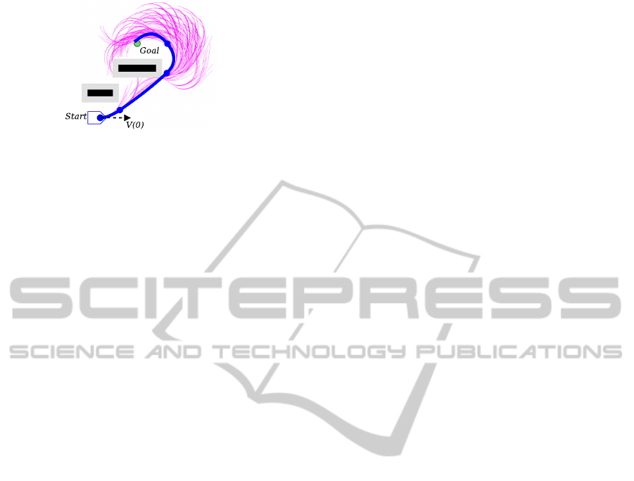
Figure 1: Example of DKP quadratics samples tree in

magenta. The ﬁnal trajectory from Start to Goal is in blue.

With its selection/propagation architecture, DKP pro-

vides properties for the low layer that we need to build

a cognitive trajectory planner. It produces trajectories

that respect the kinematic constraints of the robot and

avoid obstacles as shown in Figure 1. It also translates

steering behavioursinto parameters for the underlying

trajectory planner. Finally, it provides solutions that

optimize a criterion and it is deterministic: the cogni-

tive part should not have to repeat trajectory planning

until an optimal solution is found if one exists.

The steering tree is made up of instantiated

models of HTN (Hierarchical Task Networks) sub-

trees representing steering behaviours. Common ap-

proaches are based either on a STRIPS-like descrip-

tion of the world and possible actions, or on HTN

decomposition of goals into compound tasks. HTN

have been widely used because they allow a human-

friendly description of tasks, even if their practical ex-

pressiveness is not better than STRIPS (Lekavy and

N´avrat, 2007). We use TÆMS (Decker, 1996), which

is a formalism used to describe HTN, to describe

complex tasks using resources, having durations and

complex interrelations, which is the case in robotic

applications.

So, our approach combines top-down and bottom-

up interactions. The latter provides a way for the bot-

tom layer, DKP, to give information to a cognitive top

layer, using TÆMS, allowing it to decide which ac-

tion to take based on different evaluable alternatives.

The paper is organized as follows. Section 2 details

our two-layer architecture. Sections 3 and 4 give two

examples demonstrating the beneﬁts of our architec-

ture for roadmap-based guidance and for the evalua-

tion of various steering behaviours in an overtaking

scenario.

2 STEERING BEHAVIOURS FOR

TRAJECTORY PLANNING

We propose to create a steering behaviour driven tra-

jectory planner. Two trees grow in parallel: a steer-

ing behaviour tree and a trajectory tree, following the

model in (Reynolds, 1999). The steering behaviour

tree controls the trajectory tree growth and DKP in-

ternal selection/propagation properties, following the

trajectory tree state. The trajectory tree created by

DKP grows if possible in the environment and trig-

gers the instantiation of new behaviours in the steer-

ing behaviour tree in reaction to situations encoun-

tered in the environment. The steering behaviour tree

reﬂects the trajectory tree: each steering behaviour

corresponds to a valid subtree of the DKP trajectory

tree if this steering behaviourrespects the dynamics of

the robot. Finally, this steering behaviour tree is used

to select the chain of behaviours to follow using the

TÆMS formalism. Our architecture can be seen as a

roadmap based planner where waypoints are replaced

by steering behaviours situated in the environment.

2.1 Controlling DKP with Steering

Parameters

In DKP, all trajectory planning constraints c such

as kinematic constraints and obstacles avoidance con-

straints require a geometrical representation S

c,tr

(t),

moved along tr

(t) for mobile obstacles. DKP also

needs the transformations T

from the constraint basis

to the parameter space basis and back. Finally, a con-

straint c is the tuple (S

c,p

(t),T

). Let C = {c

} denote

the set of constraints applied to a sample.

We deﬁne a goal guidance for propagation level

by the tuple (A

Goal,tr

Goal

(t),Goal) which associates a

Goal state to a delimited zone of the environment

Goal,tr

Goal

(t), represented with constructive surface

geometry approach, moved along tr

Goal

(t). The prop-

agation part of DKP extends an exploration tree in the

environment. When the end point of a selected sam-

ple p

...k

(t) is contained in A

Goal,tr

Goal

(t), the next

grown samples minimize the distance to the associ-

ated Goal in the propagation level. A set of propa-

gation goal guidances is denoted PGuide and A

PGuide

is the set of areas which are associated to a goal

within a set of goal guidances. We require that the

areas from A

PGuide

do not overlap: A

Goal,tr

Goal

(t) ∩

Goal,tr

Goal

(t) =

0 with k 6= l.

With the same formalism than propagation goal

guidance, we deﬁne goal guidance for selection level

with a set denoted SGuide. These goals work sepa-

rately from the propagation level to guide the explo-

ration tree created by the selection level. Only one

goal may be deﬁned to keep the good properties from

the selection process (which works in an A

∗

manner).

Time properties in propagation level are T

min

the minimal sample duration; T

max

, the maximal

sample duration and Sample

step

, the time interval

ICAART 2012 - International Conference on Agents and Artificial Intelligence

120

in order to produce samples of duration T

min

Sample

step

,...,T

max

. A discretisation step step is set

for evaluating constraints in the propagationlevel. So,

the tuple T

= (T

min

max

,Sample

step

,step) describes

the inherited time properties of the samples in the

exploration tree. In the backtracking mode used for

this paper, only one sample is created for each prop-

agation step: Sample

step

= 0 and T

min

= T

max

. The

time discretisation for constraints evaluation is set to

step = T

max

/10.

An area parameters set sp is the tuple

sp,tr

(t),C

,PGuide

,SGuide

prop

) associating

to an area A

sp,tr

of the workspace W some steering

parameters: a set of constraints C

, a set of goal

guidance for the propagation level PGuide

, a set of

goal guidance for the selection level SGuide

and the

time properties T

. The steering parameters set, de-

noted SP, contains all the area parameters sets. Let

be the set of areas that are associated to steering

parameters.

2.2 Simultaneously Growing Trees

The complete steering behaviour tree is built using

automatic instantiation of subtree models represent-

ing the steering behaviour library of the application.

We use the TÆMS formalism (Horling et al., 1999).

Even if our architecture does not limit the usage of

any of the TÆMS quality accumulation functions, in

this paper, we only use two of them:

• q seq sum used when all the subtasks need to be

completed in order before giving a quality to the

supertask. In this case, the supertask will get the

combined quality of all its subtasks as its quality;

• q max, which is functionally equivalent to an OR

operator. It says that the quality of the supertask

is equal to the maximum quality of any one of its

subtasks.

We propose an area triggering system to apply

steering behaviours on the exploration tree: each node

in the TÆMS tree contains a steering parameter set

SP associated to an area set A

. When the end-

ing point of a selected sample p

...k

(t) in the DKP

tree is contained in A

,tr

(t), this sample is prop-

agated using the steering parameters from sp

, over-

riding the previous area parameters set sp

k−1

which

ruled the guidance of the exploration tree until this

sample. It means that other samples not concerned

by this triggering will pursue using their respective

steering parameters. When applied, the next samples

in the exploration tree also inherit sp

until new steer-

ing parameters are applied on one of the next samples

and so on. When only one area from A

can be trig-

gered as a successor of an area parameters set sp

0,...,k

we create a q seq sum node in the TÆMS tree with

two children: the ﬁrst one contains the area parame-

ters set sp

0,...,k

and the second one contains the next

area parameters set sp

0,...,k,k+1

. If an area parame-

ters set sp

0,...,k,k+1,k+2

can be triggered as a successor

of the area parameters set sp

0,...,k,k+1

, sp

0,...,k,k+1,k+2

is added to the q seq sum node. When n areas from

can be triggered as successors of an area parame-

ters set sp

0,...,k

, we create a q max node in the TÆMS

tree with n children containing the associated area pa-

rameters sets. This q max node is added as a child

to the q seq sum node containing sp

0,...,k

. When the

end point of a selected sample p

...k

is contained in

sp,p

(t), the next grown samples of the exploration

tree are created respecting the corresponding set of

constraints C

sp,k

and using the corresponding set of

goal guidance for the propagation level PGuide

sp,k

goal guidance for the selection level SGuide

sp,k

and

the time properties of the exploration tree.

The DKP exploration tree interacts closely with

the steering behaviour tree thanks to the area trigger-

ing system. When the end point of a selected sample

...k

is contained in n areas A

sp,tr

(t), we create n

independent new forks in the DKP tree. We can see

each fork as a new DKP exploration subtree with the

sample p

...k

as root, each ﬁrst sample child apply-

ing one of the n steering parameter sets. Nevertheless,

some samples may overlay in the workspace, espe-

cially those near the root sample p

...k

from which

the n different steering parameters sets are expanded.

3 ILLUSTRATIVE EXAMPLES:

ROADMAP-BASED GUIDANCE

We use the environment of Figure 1 for this ﬁrst ex-

ample which illustrates the use of the steering tree to

guide the trajectory planning algorithm on a roadmap.

A roadmap captures the connectivity of the different

areas of the environment. It is made up of precom-

puted paths allowing the mobile robot to explore the

environment while avoiding obstacles.

Among the numerous existing approaches pro-

posed in literature, we opted for a Voronoi diagram

because it has the property of keeping the robot away

from obstacles: the paths composing the roadmap

are equidistant to obstacles boundaries. This obstacle

clearance property naturally provides a good roadmap

to guide the robot. It also let it substantially deviate

from it because the area around the roadmap is free.

An example of roadmap generated with a Voronoi

diagram is provided in Figure 3(a) (thick light grey

lines). This is done in two steps. First, the contours of

obstacles and of the environment bounds are discre-

TOWARDS COGNITIVE STEERING BEHAVIOURS FOR TWO-WHEELED ROBOTS

121

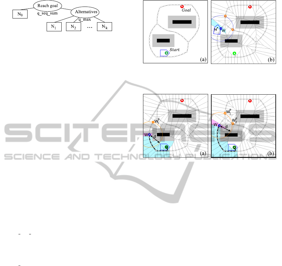
Figure 2: The TÆMS crossroads pattern to be instantiated

in the steering tree.

tised to obtain a set of points from which we generate

a Voronoi diagram. Second, the Voronoi diagram is

simpliﬁed by removing the segments crossing obsta-

cles or going to the boundary of the environment.

To perform the guidance of the robot over the

roadmap, we have to retrieve the nearest waypoint

W in the roadmap to any potential location M of the

robot in the environment. This can be efﬁciently done

by building a meta Voronoi diagram: a Voronoi di-

agram around the Voronoi diagram waypoints. We

obtain a polygonal decomposition of the environment

illustrated in Figure 3(b) (thin black lines). Each poly-

gon P contains a unique waypoint W of the roadmap.

The area of P contains all the points of the environ-

ment closer to W than the other waypoints. We see

in Figure 3(b) that from a robot location M, we can

retrieve the containing polygon P (ﬁlled in magenta)

and then the associated waypoint W (plotted in blue).

Using this cellular decomposition, we can build

the steering tree making the bridge between the tra-

jectory planner and the roadmap. The steering tree

models all the possible strategies to bypass the obsta-

cles. A bypassing strategy can be modelled by the

TÆMS crossroads pattern illustrated in Figure 2:

• the q seq sum node expresses the trajectory has

not reached the goal and has to be continued. The

node corresponds to the part which has already

been done and for which we have an evaluation.

• the q max node chooses the best alternative (i.e.

the alternative of maximal quality) between the

steering behaviour subtrees N

, ..., N

, that is, the

best bypassing strategy among k.

The steering tree is made up of instantiated cross-

roads patterns. It is progressivelybuilt thanks a depth-

ﬁrst traversal of the roadmap, from the Start way-

point. Each time a waypoint W of the roadmap is

visited, it is projected at a given distance d on the

roadmap. This projection consists in ﬁnding on the

roadmap the k waypoints W

, (i ∈ {1, k}) situated at

least at the distance d from W. This is depicted in

Figure 4 where projected waypoints are plotted in or-

ange. Note that if the projected waypoint has already

been visited, it is ignored.

This notably forbids to go backward and perform

loops. This can be observed in Figure 4, where vis-

ited waypoints are illustrated through their associated

Figure 3: (a) A roadmap as a simpliﬁed Voronoi diagram

(thick grey lines). (b) Meta Voronoi diagram (thin black

lines) associating a unique area to each roadmap waypoint.

Figure 4: Roadmap waypoint W associated to a robot posi-

tion M, and projected waypoints W

at a distance d. (a) 1

projected waypoint, on 1 branch, before the crossing, (b) 2

projected waypoints, on 2 branches, after crossing.

area, depicted in cyan. For instance, for the W way-

point from Figure 4(a), there would be two theoretical

projected waypoints: W

(above W) and W

(below

W), but W

is not considered.

When creating steering parameter set SP

associ-

ated to steering node N

, two cases are possible. First,

if the projection process leads to a unique projection

waypoint (k = 1), the pair (P,W

) is added to the set

of goal guidance for the propagation level PGuide

sp,k

Second, when several projected waypoints are de-

tected (k > 1), a crossing in the roadmap has been

passed and the considered polygons P are identiﬁed

as triggering areas A

sp,k

for each k new steering pa-

rameters set SP

i+k

. In this case, a new crossroads

pattern is instantiated in the steering tree, associating

the new steering parameter sets to TÆMS nodes and

generating new alternatives to be evaluated.

Figure 5 shows the steering tree associated to the

environment of Figure 4. This steering tree allows

the trajectory tree of Figure 6 to evaluate the 4 pos-

sible steering behaviours, by planning the 4 associ-

ated trajectories (drawn in blue). The distance d used

to project waypoints on the roadmap directly impacts

the smoothness of the trajectories, allowing smooth

turns in places where the roadmap has sharp corners.

Generated trajectories are guaranteed to be feasible by

the robot and contain its required speed for all points,

ICAART 2012 - International Conference on Agents and Artificial Intelligence

122

which is not the case of the initial Voronoi based

roadmap. Once all the alternatives are known, the

best one can be chosen, according to an application-

dependent criterion (e.g. curvature, length, time or

energy spent).

If we compare the DKP tree of Figure 1 to the one

of Figure 6, we can see that the shape of the ﬁnal tra-

jectories are better than when DKP runs alone. The

tree also contains much lesser branches, resulting in

faster computation, even with better environment ex-

ploration.

4 ILLUSTRATIVE EXAMPLES:

OVERTAKING

Description. For this example, we consider the fol-

lowing scenario, illustrated by Figure 9. A fast robot

moves as fast as possible on a road-like environ-

ment with two lanes. Robot R

starts moving at the

beginning of the bottom lane and wants to go to the

extremity of this lane. A slower robot R

also moves

straight on the bottom lane at a constant speed S

. In

the top lane, another robot R

also moves at a con-

stant speed S

= S

, in the opposite direction. The

road is 500m long and 6m wide. Robot dimensions

are 4m×1.7m (like a small car). The clearance on the

robot sides is set to 1.15m. Robots R

and R

move

at a speed of 110 km/h (∼ 30m/s) on their respective

lanes. R

must reach an overall goal G

(t) set at the

end of the bottom lane (main goal set in SGuide).

As shown in (Gaillard et al., 2011), DKP can deal

with this kind of overtaking situation. From our point

of view, the solution (the one from DKP used alone

or solutions from other hybrid trajectory planners) is

a ”forward obstacle avoidance”: there is no reason-

ing or adaptation about the kinematic constraints or

the samples duration during the trajectory planning

(except for the backtracking process). The kinematic

constraints are too low to apply to a common overtak-

ing situation that we may meet on our roads. More-

over, even if the kinematic constraints may allow an

overtake, if the robot R

starts too close, DKP may

fail to provide an intuitive ”wait and follow” solution:

in DKP, the trajectory is forced to move as far as pos-

sible because of the distance minimizing criterion.

Using steering behaviours, we can deal with this

situation with more realistic parameters. This al-

lows to get and evaluate both follow and overtake be-

haviours. We ﬁrst set the initial following steering be-

haviour for the robot R

. To reach the Goal G

(t), R

cruises fast at a maximum speed of 130 km/h: the lin-

ear speed constraint is set to [30,36]m/s, time samples

are set to 0.5s and G

(t) is added to SGuide.

When R

catches up with R

, i.e. enters in area

(t) behind R

, it triggers the instantiation of the fol-

low or overtake steering behaviour. Two alternatives

are set under a q max node and are added to the steer-

ing tree. R

may adjust its speed to R

one and fol-

low it: the linear speed constraint is set to [27,30]m/s,

time samples are set to 1s (following a robot cruising

at a constant speed does not require very reactive ma-

noeuvres) and G

(t) stays the goal. R

may overtake

and this behaviour is factorised under a q seq sum

node. The overtake steering behaviour uses different

steering parameters sets:

1. R

accelerates to 150km/h and goes to top lane:

the linear speed constraint is set to [30,42]m/s,

time samples are set to 0.1s (overtaking requires

a precise driving at this speed) and a goal G

(t)

added to PGuide enforces R

to turn left.

2. when R

enters in area A

(t) behind R

on the top

lane, in the same speed conditions, it stays on top

lane: a goal G

(t) added to PGuide is set at the

end of the top lane.

3. when R

enters in area A

(t) in front of R

on the

top lane, in the same speed conditions, it goes to

the bottom lane: a goal G

(t) added to PGuide

enforces R

to turn right.

4. when R

enters in area A

(t) in front of R

on the

bottom lane, it returns to the cruise steering be-

haviour.

Figure 7 shows the steering tree of this example. The

areas and goals associated to the motion of R

are il-

lustrated in Figure 8

The trajectory planning returns a solution associ-

ated to each behaviour. For instance, in Figure 9(a),

the overtake behaviour is not solved when the robot

sits in the opposite lane at the same instant: only

the follow behaviour should be applied as valid trajec-

tory. If R

sits further (Figure 9(b)), the overtake be-

haviour is also solved and should be applied as valid

trajectory. The overtake behaviour solution lasts 13s

whereas the follow behaviour solutions lasts 15.5s.

Once again, the resulting trajectories are better than

with DKP alone. The trajectory tree is also far less

complex than usual solutions from DKP, where a lot

of backtrack occurs before a valid trajectory is found.

Computation time is thus greatly reduced.

We presented two possible usages of our archi-

tecture, but the expressiveness of the steering pa-

rameter and TÆMS languages is high enough to de-

scribe other human-like steering behaviours. Dy-

namic changes of the acceleration or linear/angular

Figures 8 and 9 have been vertically upscaled ∼ 8

times.

TOWARDS COGNITIVE STEERING BEHAVIOURS FOR TWO-WHEELED ROBOTS

123

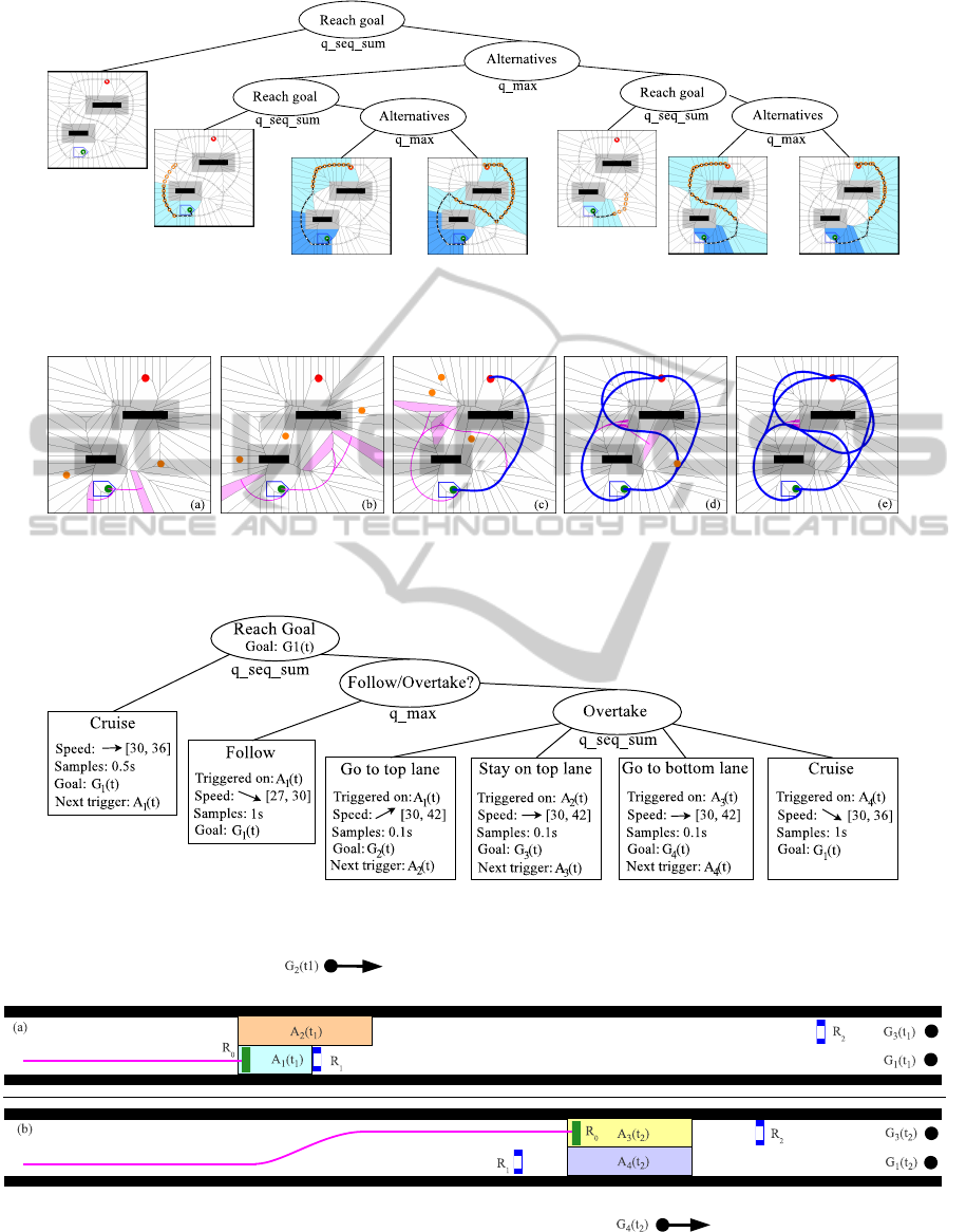
Figure 5: The steering tree for a roadmap-based guidance. Each leaf corresponds to an area, ﬁlled in cyan, in which there

is no crossing and where intermediate goals are plotted in orange. Dark blue polygons represent areas to be ignored because

they have already been visited in parent nodes.

Figure 6: The trajectory tree guided by the steering tree of Figure 5. Blue curves are the ﬁnal trajectories that reach the goal.

Magenta curves are under construction or given up trajectories. Light magenta polygons correspond to arrival areas of under

construction trajectories. Orange dots are associated intermediate goals, provided by the steering tree.

Figure 7: The ﬁnal steering tree for overtaking. Nodes with thick lines were created in the initial conﬁguration of the tree.

Other nodes come from the instantiation of the Follow/Overtake pattern.

Figure 8: Overtaking areas and goals represented at different time steps. (a) at t

, when a candidate trajectory enters the

(t) area, (b) at t

, when a candidate trajectory enters the A

(t) area. The controlled robot is the green rectangle and the

vehicles to avoid are the blue rectangles.

ICAART 2012 - International Conference on Agents and Artificial Intelligence

124

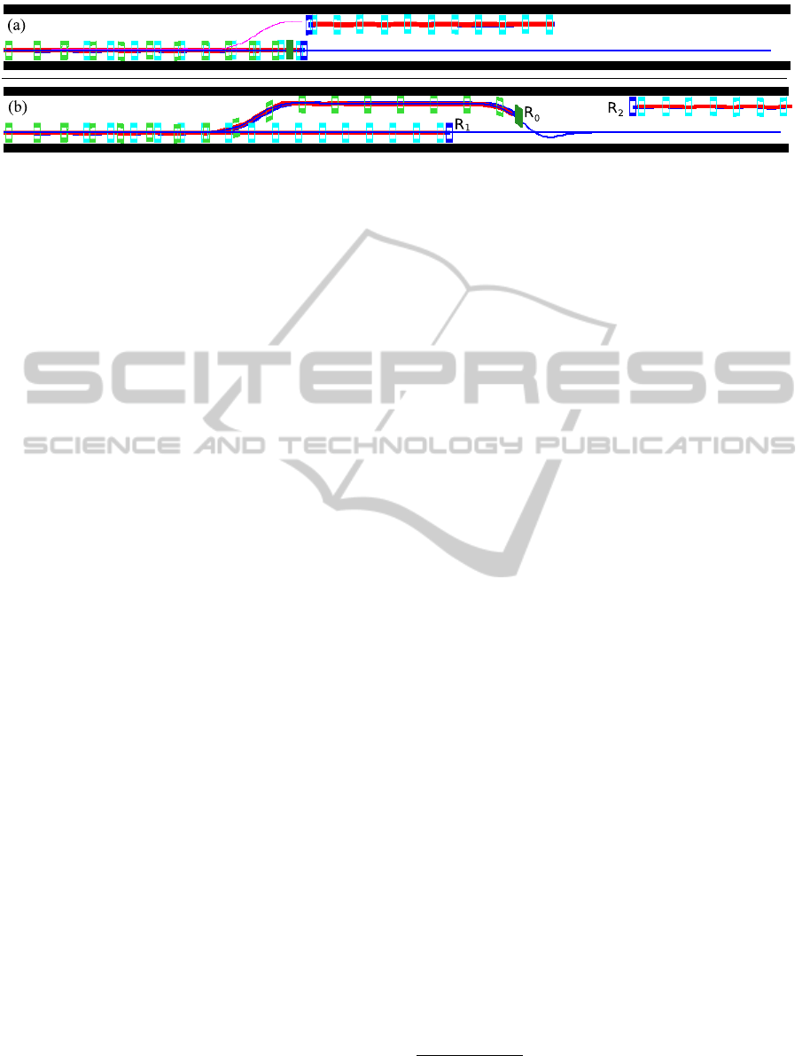
Figure 9: Different overtaking situations. (a) R

, in green, cannot overtake. It must follow R

using the trajectory in blue.

(b) R

can follow or overtake R

and we get two alternative trajectories in blue. R

is drawn on the one that overtakes.

speed constraints and of the goal point could be used

to describe other driving manoeuvres and smooth or

aggressive driving behaviours.

5 CONCLUSIONS AND FUTURE

WORKS

Like Reynolds did for autonomous characters in sim-

ulated environments, we want to introduce steering

behaviours for mobile robots but using a cognitive

rather than a reactive approach. We presented an ar-

chitecture where two tightly coupled layers are used

to co-elaborate candidate trajectories that may be

evaluated by a cognitive layer to choose the best one

to apply in a particular situation.

For the ﬁrst layer, we chose the DKP trajectory

planner which is able to efﬁciently deal with kinody-

namic constraints in a real continuous world. But, this

single layer cannot handle all the aspects governing a

good trajectory for a complex robot task. We thus

added a TÆMS based layer which role is to make the

connection between higher cognitive layers and the

trajectory planning layer. In this layer, we are able to

describe steering behaviours that constraint in a top-

down interaction the construction of the DKP trajec-

tory tree. The interaction is also bottom-up because

steering behaviours are instantiated in reaction to sit-

uations detected during the construction of the trajec-

tory tree. Detailed examples showed that this archi-

tecture is also more efﬁcient for the solution explo-

ration than DKP alone.

Future works will focus on two main improve-

ments of this architecture. First, its ability to run con-

tinuously. For the moment, we have to launch distinct

successive planning tasks to deal with an endless sce-

nario. We may continuously grow our two trees to re-

act to new events, select nodes to execute and discard

already executed nodes. Second, we will work on a

third layer reasoning about the steering behaviours

to instantiate them for the achievement of the high

level goals of the robot and to possibly merge them.

We would be allowed to generate and evaluate com-

pound behaviours like overtake aggressively or follow

smoothly.

REFERENCES

Branicky, M., Curtiss, M., Levine, J., and Morgan, S.

(2006). Sampling-based planning, control and veri-

ﬁcation of hybrid systems. IEE Proceedings Control

Theory and Applications, 153(5):575.

Decker, K. (1996). TÆMS: A Framework for Environment

Centered Analysis & Design of Coordination Mech-

anisms. Foundations of Distributed Artiﬁcial Intelli-

gence, Chapter 16, pages 429–448.

Gaillard, F., Soulignac, M., Dinont, C., and Mathieu, P.

(2010). Deterministic kinodynamic planning. In Pro-

ceedings of the Eleventh AI*IA Symposium on Artiﬁ-

cial Intelligence, pages 54–61.

Gaillard, F., Soulignac, M., Dinont, C., and Mathieu, P.

(2011). Deterministic kinodynamic planning with

hardware demonstrations. In Proceedings of IROS’11.

To appear.

Horling, B., Lesser, V., Vincent, R., Wagner, T., Raja, A.,

Zhang, S., Decker, K., and Garvey, A. (1999). The

TAEMS White Paper.

Jaesik, C. and Eyal, A. (2009). Combining planning and

motion planning. 2009 IEEE International Confer-

ence on Robotics and Automation.

Lacroix, B., Mathieu, P., Rouelle, V., Chaplier, J., Galle, G.,

and Kemeny, A. (2007). Towards trafﬁc generation

with individual driver behavior model based vehicles.

In Proceedings of DSC-NA’07, pages 144–154.

Lekavy, M. and N´avrat, P. (2007). Expressivity of STRIPS-

Like and HTN-Like Planning, volume 4496/2007 of

Lecture Notes in Computer Science, pages 121–130.

Springer Berlin / Heidelberg, Berlin, Heidelberg.

McDermott, D., Ghallab, M., Howe, A., Knoblock, C.,

Ram, A., Veloso, M., Weld, D., and Wilkins, D.

(1998). Pddl-the planning domain deﬁnition language.

The AIPS-98 Planning Competition Comitee.

Reynolds, C. (1999). Steering behaviors for au-

tonomous characters. In Game Developers Confer-

ence. http://www. red3d. com/cwr/steer/gdc99.

This work is supported by the Lille Catholic Univer-

sity, as part of a project in the Handicap, Dependence and

Citizenship pole.

TOWARDS COGNITIVE STEERING BEHAVIOURS FOR TWO-WHEELED ROBOTS

125