EFFICIENT TOLERANT PATTERN MATCHING WITH
CONSTRAINT ABSTRACTIONS IN DESCRIPTION LOGIC
Carsten Elfers, Stefan Edelkamp and Otthein Herzog
Center for Computing and Communication Technologies, University of Bremen, Am Fallturm 1, 28359 Bremen, Germany
Keywords:
Tolerant pattern matching, Constraint abstraction, Description logic, Constraint satisfaction.
Abstract:
In this paper we consider efficiently matching logical constraint compositions called patterns by introducing
a degree of satisfaction. The major advantage of our approach to other soft pattern matching methods is to
exploit existing domain knowledge represented in Description Logic to handle imprecision in the data and to
overcome the problem of an insufficient number of patterns. The matching is defined in a probabilistic frame-
work to support post-processing with probabilistic models. Additionally, we propose an efficient complete
algorithm for this kind of pattern matching, which reduces the number of inference calls to the reasoner. We
analyze its worst-case complexity and compare it to a simple and to a theoretical optimal algorithm.
1 INTRODUCTION
Conventional pattern matching methods determine if
a given pattern is satisfied or not. In real-world do-
mains these approaches suffer heavily from uncer-
tainty in the environment in form of typical noise or
imprecision in the data. This leads to the natural con-
clusion that matching patterns must become a matter
of degree (Dubois and Prade, 1993).
Our application area is improved network security
within Security Information and Event Management
(SIEM) systems that collect events from several intru-
sion detection sensors distributed in a computer net-
work. The typical huge amount of events collected by
a SIEM system calls for pattern matching correlation
techniques to be reduced to the most relevant ones.
Some well-known examples of rule-based approaches
are NADIR (Hochberg et al., 1993), STAT (Porras,
1993) and IDIOT (Kumar and Spafford, 1995). How-
ever, due to constantly varying attacks and varying
network configurations the pattern matching method
must deal with changing conditions. Variations can
be learned, e.g., by Pattern Mining approaches like
in MADAM ID (Lee and Stolfo, 2000). In real world
domains, the amount of reference data with detected
professional successful attacks is sparse. Therefore,
modeling patterns have been a dominating strategy in
enterprise SIEM systems like in the market-leading
system ArcSight (cf. (Nicolett and Kavanagh, 2010)).
In this paper an efficient tolerant pattern matching
algorithm is proposed, which handles variations by
exploiting ontological (or categorical) background-
knowledge in Description Logics (DL). A semanti-
cally well-defined and intuitive method is presented
to calculate the degree of matching from patterns and
data. In contrast to the similarity measurement to han-
dle noise in the matchmaking process suggested by
He et al. (2004), our approach does not require simi-
larity weights. Additionally, we extend their work by
also describing how to handle disjunctions and nega-
tions of conditions (or constraints). Previous work
that uses DL for pattern matching in the security do-
main (Undercoffer et al., 2003; Li and Tian, 2010) do
not handle variations that deviate from the modeled
patterns. We present an efficient algorithm for finding
the best tolerant matching; a critical requirement in
real-world domains.
2 PATTERN MATCHING
Our tolerant pattern matching approach is based on
constraint satisfaction in ontologies specified in DL.
It consist of concepts (classes of objects), roles (bi-
nary relations between concepts) and individuals (in-
stances of classes) (cf., (Gomez-Perez et al., 2004, p.
17)). The semantics are defined by the interpretation
(an interpretation can be regarded as the correspond-
ing domain) of the set of all concept names, the set of
all role names and the set of all names of the individ-
uals (cf., (Baader et al., 2008, p. 140)). A concept C
256
Elfers C., Edelkamp S. and Herzog O..
EFFICIENT TOLERANT PATTERN MATCHING WITH CONSTRAINT ABSTRACTIONS IN DESCRIPTION LOGIC.
DOI: 10.5220/0003720102560261
In Proceedings of the 4th International Conference on Agents and Artificial Intelligence (ICAART-2012), pages 256-261
ISBN: 978-989-8425-95-9
Copyright
c
 2012 SCITEPRESS (Science and Technology Publications, Lda.)

is subsumed by a concept D if for all interpretations
I we have C
I
⊆ D
I
. In this work, tolerant pattern
matching is realized by successively generalizing the
pattern, and determining a residual degree of satisfac-
tion.
Definition 1 (Entity, Constraint, Satisfaction). An en-
tity E is either (a) an individual, (b) a concept, or (c)
a variable. A constraint γ ∈ Γ is defined as γ = eRe
0
of
a left hand side entity e, a right hand side entity e
0
and
a relation R between these entities. It is assumed that
either e or e
0
is an individual (fixed by an observa-
tion), or a variable. A constraint γ is satisfied if there
exists an interpretation I with (eRe
0
)
I
.
Definition 2 (Partially Matching Pattern, Degree of
Matching). A pattern p consists of a set of constraints
and logical compositions among them. A partially
matching pattern p – given the data x – is a real val-
ued function with range [0, 1]. The value of such a
function is called degree of matching or matching de-
gree.
1
p(x) =



1, if p fully matches
α ∈]0,1[ if p matches to degree α
0, otherwise
Each constraint in a pattern can be expressed as a
query triple in DL. This allows an easy transforma-
tion of patterns into a query language like SPARQL,
which can be interpreted by DL reasoners. Next, a
relation ≥
g
(adapted from Defourneaux and Peltier
(1996)) describes that a constraint is an abstraction
of another constraint. We say γ
1
is more general or
equal than γ
2
(noted γ
1
≥
g
γ
2
) if for all interpretations
γ
I
2
of γ
2
there exists an interpretation γ
I
1
of γ
1
such that
γ
I
2
⊆ γ
I
1
.
Fig. 1 shows an example of a pattern p
1
with
three constraints γ
1
1
,γ
1
2
,γ
1
3
and their direct abstractions
γ
0
1
,γ
0
2
,γ
0
3
. (Superscripts enumerate different levels of
specialization. A zero denotes the most abstracted
case, while a larger number indicates an increasing
specialization, e.g., p
0
is the direct abstraction of p
1
.)
Figure 1: Pattern with constraint abstractions.
1
As we will see later, the degree of matching is deter-
mined by a fusion function F.
To abstract a pattern it is first neccessary to prop-
agate all negations to the leaves (i.e., to the constraint
triples γ) by applying De Morgan’s rules. The con-
struction of this negational normal form can be done
before abstracting a pattern or be applied to all pat-
terns in advance (even to the most specific ones).
Moreover, each constraint must be abstracted by the
following rules:
• A negated constraint is abstracted to a tautology,
since the current model of such a constraint in-
cludes all individuals except of the negated one
(e.g., γ
0
3
in Fig. 1 has changed to a tautology).
• If the entity of the abstracted constraint is a con-
cept or an individual this is replaced by a more
general concept due to the defintion of ≥
g
.
• The relation of the abstracted constraint might
have to be replaced to ensure that the set of in-
terpretations of the constraint increases, e.g., the
identity relation must be exchanged to an appro-
priate (transitive) subclass relation.
A measure θ(γ
j
,γ
k
) for constraints γ
j
and γ
k
is
assumed to quantify the similarity of an abstracted
constraint γ from the original level j to an abstract
level k. A simple example of such a measure is
θ(γ
j
,γ
k
) = 1/(| j − k| + 1). We write γ
⊥
for the origi-
nal constraint on the most specific level ⊥, and θ(γ
i
)
for θ(γ
i
,γ
⊥
). Independent of a concrete ralization,
such a measurement is assumed to be 1 if the con-
straint is not abstracted, and decreases, if the con-
straint is getting more abstract; by still being greater
than or equal to 0. This measurement can also be re-
garded as a similarity function, which says how ex-
actly γ
j
describes γ
k
, or how similar they are.
Definition 3 (Similarity, extended from Fanizzi and
d’Amato (2006) and Batagelj and Bren (1995)). A
similarity measure θ is a real-valued function into
[0,1] defined by the following properties:
• ∀γ
j
,γ
k
: θ(γ
j
,γ
k
) ≥ 0 (positive definiteness)
• ∀γ
j
,γ
k
: θ(γ
j
,γ
k
) = θ(γ
k
,γ
j
) (symmetry)
• ∀γ
j
,γ
k
: θ(γ
j
,γ
k
) ≤ θ(γ
j
,γ
j
) (identity)
• ∀ j < k : θ(γ
j
,γ
k+1
) < θ(γ
j
,γ
k
) (monotonicity)
Such similarity function values of the constraints
are combined to a matching degree of the pattern
by applying some fusion operator F(θ
1
,...,θ
n
) sim-
ilar to fuzzy pattern matching (cf., (Cadenas et al.,
2005)) to consider the semantics of the logical op-
erators while abstracting the pattern. A probabilis-
tic fusion approach is suggested by using a Bayesian
interpretation of the tree of logical operators in each
pattern as follows.
2
2
These equations naturally result from a Bayesian net-
EFFICIENT TOLERANT PATTERN MATCHING WITH CONSTRAINT ABSTRACTIONS IN DESCRIPTION LOGIC
257

Definition 4 (Fusion Function). The fusion function
F(p) of pattern p is recursively defined with respect to
some similarity function θ of constraints γ composed
by logical operators.
F(γ
i
1
∧ γ
j
2
) = F(γ
i
1
) · F(γ
j
2
)
F(γ
i
1
∨ γ
j
2
) = 1 − (1 − F(γ
i
1
)) · (1 − F(γ
j
2
))
F(¬γ
i
) =

1 − F(γ
i
), for i = ⊥
β · F(γ
i
), otherwise
F(γ
i
) = θ(γ
i
),
where β is a penalty factor to additionally penalize
the abstraction of negations, since these may have a
greater impact on the result.
The factor β may depend on the used similarity
function and the depth of the ontology. The fusion
function’s conjunction/disjunction can be regarded as
deterministic AND/OR nodes. Therefore, the condi-
tional probability table is fully specified.
The negation is interpreted differently to a cor-
responding Bayesian conditional probability table to
ensure that an increasing abstraction leads to a de-
creasing fusion function. This leads to the monotonic-
ity of F wrt. θ, which is very useful for finding the
most specific abstraction as we will see later.
With these properties a partial order of patterns
with respect to the generality of their containing con-
straints is defined. From this basis it is necessary to
find the best matching pattern, i.e., the pattern with
the biggest F. This problem can be postulated for a
pattern p containing d constraints γ
x
1
,...,γ
x
d
to find
a combination of x
1
,...,x
d
which satisfies the pattern
and maximizes F. The solution of interest is in the
Pareto front of maximum x due to the monotonicity
of F with respect to θ and the monotoncity of θ itself
(cf. Def. 3). If the level of specialization increases,
F increases as well, or – in other words – if any con-
straint of the pattern is abstracted, F decreases.
3 ALGORITHM PARETO
In this section a divide-and-conquer algorithm is pro-
posed to efficiently search for the most specific sat-
isfied patterns, building the Pareto front of the con-
straint abstractions. Each level of abstraction of a
constraint is represented as one dimension of the
search space. The search space X = {0,. . . ,n −
1}
d
is divided into satisfied elements (satisfied con-
straint combinations) X
+
⊆ X and unsatisfied ele-
ments X
−
⊆ X with X
+
∩ X
−
=
/
0.
work (except of the negation) with cond. probability tables
equal to the truth table of the corresp. logical operators.
Figure 2: Example of the Pareto algorithm.
Fig. 2 gives an example how the algorithm works
for the 2D case (i.e., for γ
1
and γ
2
). At first the mid-
dle of the search space is determined, i.e., point (4,4).
Around this point the search space is divided into (in
the 2D case) four equal sized areas each including the
middle and the corresponding border elements. Two
of these areas are marked with a gray background the
others are area A and area B. The minus sign at (4,4)
indicates that the pattern with γ
4
1
and γ
4
2
is unsatisfied,
the circle indicates an inference call to test this sat-
isfaction. Therefore, all more specific pattern combi-
nations are omitted in the further recursion, i.e., area
A. This method is continued for the gray areas but at
first for area B. Area B is divided into four equal sized
areas around the middle (2,2). This is a match, there-
fore, we know that each more abstract pattern than γ
2
1
,
γ
2
2
is also matching (or satisfied), marked as area C
which can be omitted in the following. The recursion
is continued for the new middle (3, 3). At this point
an unsatisfied area can be determined which also af-
fects the currently not investigated gray areas due to
we know that from (3,3) to (8,8) every solution must
be unsatisfied because they are more or equal spe-
cific. These temporary results are stored in a list and
checked before investigating the gray areas in subse-
quent recursion steps to omit inference calls for these
points.
The algorithm can be limited in the search space
(by limiting the search depth) to give approximate re-
sults. By increasing the search depth the solution is
more and more appropriately approximated.
Algorithm 1 shows the implementation of the ap-
proach. This is initialized with an empty set of so-
lutions (representing the most specific satisfied pat-
terns) S
+
and S
−
(representing the most abstract un-
satisfied patterns). The individual search spaces are
specified by a most specific bound (msb) and a most
abstract bound (mab), where msb and mab are coor-
dinates of the search space. Initially, for all i we have
msb
i
= 0 and mab
i
= n (to ensure completeness mab
is located outside of the actual search space). For
ICAART 2012 - International Conference on Agents and Artificial Intelligence
258

Algorithm 1: Pareto.
Input: msb,mab ∈ X = {x
1
,··· ,x
d
}
d
1: m = b(mab + msb)/2c
2: if ∃x ∈ S
+
with(m ≥
g
x) then
3: s = true
4: else
5: if ∃x ∈ S
−
with(m ≤
g
x) then
6: s = false
7: else
8: s = Eval(m)
9: if s = true then
10: S
+
= {x ∈ S
+
∪ {m} | ∀x
0
∈ S
+
∪ {m} : x
0
≥
g
x}
11: else
12: S
−
= {x ∈ S
−
∪ {m} | ∀x
0
∈ S
−
∪ {m} : x
0
≤
g
x}
13: if mab = m then
14: return
15: if s = true then
16: Pareto(msb, m)
17: else
18: Pareto(m, mab)
19: for each h ∈ Hypercubenodes(msb,mab) do
20: for i = 1 to d do
21: msb
0
i
= max{h
i
,m
i
}
22: mab
0
i
= min{h
i
,m
i
}
23: Pareto(msb
0
,mab
0
)
reasons of simplicity, each constraint is assumed to
have an equal amount of specializations/abstractions,
however, the algorithm is also capable of differing
amounts.
Besides Eval, the call to the reasoner, Hy-
percubenodes(msb, mab) enumerates the sublattices
(without msb, mab themselves); formally defined as
2
d
−2
[
i=1
msb ⊗ bin(i) + mab ⊗ bin(i),
where bin(i) denotes the binary representation of a
number i, bin(i) denotes its (bitwise) complement,
and ⊗ the bitwise multiplication of two vectors.
The definition for ≥
g
in the d dimensional search
space X is given by:
Definition 5 (Domination). Let
≥
g
= {(x,x
0
) ∈ X
2
| ∀i

x
i
≤ x
0
i

}.
We say that x ∈ X
−
dominates x
0
∈ X if x
0
≤
g
x and
x ∈ X
+
dominates x
0
∈ X if x
0
≥
g
x.
All patterns more specific than an unsatisfied one
are still unsatisfied and all patterns more general than
a satisfied one are still satisfied. In other words, we
have ∀x ∈ X
−
,x
0
∈ X.(x
0
≤
g
x) ⇒ x
0
∈ X
−
and ∀x ∈
X
+
,x
0
∈ X.(x
0
≥
g
x) ⇒ x
0
∈ X
+
.
Definition 6 (Pareto Frontier). The Pareto frontier is
the set of extreme points E = E
+
∪E
−
with E
+
∩E
−
=
/
0 containing each element of X
+
with no element in
X
+
being more general
E
+
= {x ∈ X
+
| ∀x
0
∈ X
+

x
0
≥
g
x

} (1)
and each element of X
−
with no element in X
−
being
more specific
E
−
= {x ∈ X
−
| ∀x
0
∈ X
−

x
0
≤
g
x

}. (2)
No element in E is dominated by another element
in this set, i.e., the compactest representation of the
set of satisfied / unsatisfied solutions.
Next, we show that Algorithm 1 computes E
+
.
Theorem 1 (Correctness and Completeness of Algo-
rithm 1). The algorithm determines the whole set of
satisfied constraints, i.e., E
+
= S
+
.
Proof. (Correctness) To show the correctness of the
algorithm we ensure that each element of the expected
result set E
+
is in the solution set S
+
of the algorithm
and, vice versa, i.e., e
+
∈ E
+
⇒ e
+
∈ S
+
and s
+
∈
S
+
⇒ s
+
∈ E
+
.
Lemma 1. (s
+
∈ S
+
⇒ s
+
∈ E
+
)
If the search is exhaustive (this is shown later)
Line 10 implies that s
+
∈ S
+
⇒ s
+
∈ E
+
, since it com-
putes S
+
as {x ∈

S
+
∪ {m}

| ∀x
0
∈

S
+
∪ {m}

:
x
0
≥
g
x}, which is the same as the expected result E
+
with S
+
∪ {m} ⊆ X
+
.
Lemma 2. (e
+
∈ E
+
⇒ e
+
∈ S
+
)
We investigate four conditions under which an el-
ement is inserted into (and kept in) the solution set of
the algorithm S
+
. These conditions, directly derived
from the algorithm, are as follows
1. Each element from S
+
must be contained in X
+
which is exactly the same condition as in defini-
tion of E
+
.
2. The following assumption derived from Lines 2
and 4, must hold for e
+
to be inserted into S
+
¬∃x
0
∈ S
+
.

e
+
≥
g
x
0

.
This condition is not fulfilled if an equivalent solu-
tion e
+
is already in the set S
+
or if e
+
dominates
another element from S
+
. In both cases e
+
is not
inserted into the result set S
+
.
3. The next statement, derived from Line 5 and 7, is
¬∃x
0
∈ S
−
.

e
+
≤
g
x
0

. (3)
This condition is always fulfilled, since we con-
sider the case that e
+
∈ X
+
which implies that x
0
∈
X
+
which cannot be the case since x
0
∈ S
−
⊆ X
−
.
4. Line 10 does not drop solutions because for all
m ∈ X
+
we have Eqn. 1.
Analogically, the proof can be made for E
−
.
Proof. (Completeness)
Recursion is omitted for
EFFICIENT TOLERANT PATTERN MATCHING WITH CONSTRAINT ABSTRACTIONS IN DESCRIPTION LOGIC
259

• {x ∈ X | msb ≤
g
x ≤
g
m} if m ∈ X
−
and for
• {x ∈ X | m ≤
g
x ≤
g
mab} if m ∈ X
+
.
This does not affect the set of solutions due to the def-
inition of domination and the definition of E that there
should not be any value in the result set that is dom-
inated by another element. Note that m has already
been checked by the algorithm at this point.
The remaining space under investigation is getting
smaller in each recursion path until m is getting equal
to mab (termination criterion in Line 13). This is only
the case if each edge of the space under investigation
is smaller or equal one (Line 1). At some time in the
recursion the space of possible solutions is divided
into a set of spaces with edges of the length one or less
by still covering the whole space of possible solutions
as previously shown. Further, if any point of such a
smallest area is a possible solution (these are the cor-
ners), this point is under investigation in another space
due to the recursive call with overlapping borders ex-
cept of the borders of the whole search space at the
specific borders due to there is no mab of any area
including these specific border elements, e.g., there is
no mab for the one element area (8, 8) in the exam-
ple from Fig. 2. For this border case the algorithm
is called with a lifted msb to ensure that the unlifted
specific bound is included in some smallest (one el-
ement) area as mab visualized as a light gray border
in Fig. 2. Therefore, each element of the search space
which is a possible solution is investigated as a mab
in some recursive path.
After computing the Pareto front, the fusion func-
tion F identifies the most specific matching pattern
abstraction in the remaining set of candidates
We observe that the (worst-case) running time
complexity is dominated by the number of calls to
the DL reasoner. In the following analysis, we dis-
tinguish between the number of recursive calls T (n)
and the number of inference calls C(n) (for the sake
of simplicity, we assume n
1
= ... = n
d
and n = 2
k
).
Of course, a trivial algorithm testing all possible ele-
ments in S induces C(n) = T (n) = O(n
d
). We will see
that the algorithm Pareto is considerably faster.
With lg n we refer to the dual logarithm log
2
n,
while lnn refers to the natural logarithm log
e
n.
Recursive Calls. For the 2D case, the number of calls
of the divide-and-conquer algorithm in a 0/1 (n × n)
matrix is bounded by
T (k) =
k
∑
i=0
3
i
=

3
k+1
− 1

/2
Assuming n = 2
k
we have
T (n) =

3
lgn
− 1

/2 =

n
lg3
− 1

/2 = O(n
1.5849
)
For larger dimensions d the complexities
O(n
lg(2
d
−1)
) rise.
Inference Calls. For the 2D case the structure of
the recursion corresponds to find a binary search to
the SAT/UNSAT boundary. The recursion depth is
bounded by lg n. Therefore, the worst-case number of
calls to the reasoner of the algorithm in a 0/1 (n × n)
matrix is defined by
C(n) = 2C(n/2) + O(lg n).
The O(lgn) term is due to the binary search. In the
worst case the boundary between SAT and UNSAT
cells is in the middle, where one quarter of SAT and
one quarter of UNSAT elements are omitted.
Using the Akra-Bazzi theorem (Akra and Bazzi,
1998), the above recursion can be shown to reduce
to C(n) = O(n) as follows. For k = 0 it states that
for recurence equation T (n) = g(n) + aT (n/b) with
a = b
p
we have the following closed form
T (n) = O

n
p
·

1 +
Z
n
1
g(u)/u
p+1
du

.
Here, g(n) = lgn = ln n/ ln 2 and a = b = 2 so that
p = 1 and
T (n) = O

n + n ·
Z
n
1
ln(u)/u
2
du

= O(n + n · [− lnu/u]
n
1
) = O(n).
For larger dimensions d the complexities
O(n
lg(2
d
−2)
) rise.
4 EVALUATION
We have evaluated the efficiency of the algorithm with
respect to the number of inference calls. In Fig. 3
two tolerant matching algorithms and the result of a
perfect guessing algorithm (a lower bound) are visu-
alized. It is assumed that the lower bound algorithm
checks exactly the Pareto border of satisfied and un-
satisfied elements. Therefore, the best possible algo-
rithm needs at least |S
+
| + |S
−
| inference calls.
The proposed divide-and-conquer algorithm
Pareto with pruning the recursive calls as in Algo-
rithm 1 – but without using the lists S
+
and S
−
–
is called Pareto-0. This is the first efficient algo-
rithm one might think of. The proposed algorithm
is visualized as Pareto and the lower bound as
LOWERBOUND for the 2D case in Fig. 3 (no log-
scale) and for the 4D case in Fig. 4 (log-scale). The
x-axis represents the amount of possible abstractions
and the y-axis the amount of reasoner calls.
ICAART 2012 - International Conference on Agents and Artificial Intelligence
260

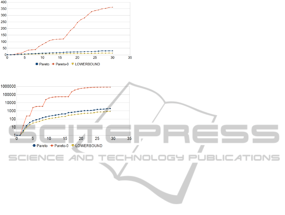
Figure 3: DL Reasoner calls in the 2D case.
Figure 4: DL Reasoner calls in the 4D case with logarithmic
scaling.
Both figures show that the inference calls of
Pareto is near to the optimal lower bound LOWER-
BOUND and considerably better than the typical
divide-and-conquer algorithm Pareto-0 in both 2D
and 4D. These results are reasonable for the proposed
pattern matching algorithm due to the depth of an on-
tology being typically smaller than 30 and the patterns
having typically a small amount of constraints.
We see that the amount of Pareto results, which
is around the half of the LOWERBOUND value, is
very small. For this set the degree of matching must
be computed with respect to the fusion function to
find the most optimal solution out of the set of Pareto-
optimal solutions. This search can be done without to
call the DL reasoner, since we already know that these
solutions are satisfied.
5 CONCLUSIONS
We have shown how to use ontological background
DL knowledge to overcome the problem of noisy and
imprecise data. Our tolerant pattern matching ap-
proach can even address erroneous or missing patterns
by successively abstracting them. The algorithm sub-
stantially reduced the amount of these inference calls
to the DL reasoner. It is correct, complete and needs
a number of inference calls close to the lower bound.
It can be parameterized to have the ability to infere
approximate results.
ACKNOWLEDGEMENTS
This work was supported by the German Federal Min-
istry of Education and Research (BMBF) under the
grant 01IS08022A.
REFERENCES
Akra, M. and Bazzi, L. (1998). On the solution of linear re-
currence equations. Computational Optimization and
Applications, 10(2):195–210.
Baader, F., Horrocks, I., and Sattler, U. (2008). Handbook
of Knowledge Representation. Elsevier.
Batagelj, V. and Bren, M. (1995). Comparing Resemblance
Measures. Journal of Classification, 12(1):73–90.
Cadenas, J. M., Garrido, M. C., and Hernndez, J. J. (2005).
Heuristics to model the dependencies between fea-
tures in fuzzy pattern matching. In EUSFLAT.
Defourneaux, G. and Peltier, N. (1997). Analogy and ab-
duction in automated deduction. In IJCAI.
Dubois, D. and Prade, H. (1993). Tolerant fuzzy pattern
matching: An introduction.
Fanizzi, N. and d’Amato, C. (2006). A similarity measure
for the ALN description logic. In CILC, pages 26–27.
Gomez-Perez, A., Fernandez-Lopez, M., and Corcho, O.
(2004). Ontological Engineering. Springer.
He, Y., Chen, W., Yang, M., and Peng, W. (2004). Ontol-
ogy based cooperative intrusion detection system. In
Network and Parallel Computing, pages 419–426.
Hochberg, J., Jackson, K., Stallings, C., McClary, J.,
DuBois, D., and Ford., J. (1993). Nadir: An auto-
mated system for detecting network intrusion and mis-
use. Computers & Security, pages 235–248.
Kumar, S. and Spafford, E. H. (1995). A Software Architec-
ture to support Misuse Intrusion Detection. In NISC,
pages 194–204.
Lee, W. and Stolfo, S. J. (2000). A framework for con-
structing features and models for intrusion detection
systems. ACM Transactions on Information and Sys-
tem Security, 3:227–261.
Li, W. and Tian, S. (2010). An ontology-based intrusion
alerts correlation system. Expert Systems with Appli-
cations, 37(10):7138 – 7146.
Nicolett, M. and Kavanagh, K. M. (2010). Magic quadrant
for security information and event management.
Porras, P. (1993). STAT – a state transition analysis tool for
intrusion detection. Technical report, UCSB, USA.
Undercoffer, J., Joshi, A., and Pinkston, J. (2003). Mod-
eling computer attacks: An ontology for intrusion de-
tection. In RAID, pages 113–135.
EFFICIENT TOLERANT PATTERN MATCHING WITH CONSTRAINT ABSTRACTIONS IN DESCRIPTION LOGIC
261