
AN OPEN SOURCE TOOL FOR HEART RATE VARIABILITY
WAVELET-BASED SPECTRAL ANALYSIS
Constantino A. Garc´ıa
1
, Abraham Otero
1
, Xos´e Vila
2
and Mar´ıa J. Lado
2
1
Department of Software and Knowledge Engineering, University San Pablo CEU, 28668 Madrid, Spain
2
Department of Computer Science, University of Vigo, Campus As Lagoas s/n, 32004 Ourense, Spain
Keywords:
Heart Rate Variability, Wavelet Transform, RHRV.
Abstract:
Heart rate variability (HRV) power spectrum analysis is a well-known technique used to study the activity
of the autonomic nervous system. It is performed by calculating the spectral power of certain bands of the
RR time series. There are several tools that perform this type of analysis: Kubios HRV, PhysioNet’s HRV
toolkit for MatLab and aHRV, among others. All these tools use the Short Fourier Transform to estimate
spectral power. However, the RR time series is a non-stationary signal. The Wavelet transform is often a more
suitable tool for analyzing non-stationary signals than the Short Time Fourier Transform. Its usefulness in
HRV analysis has already been proven in the literature. However, the lack of HRV analysis tools that support
it has made this technique underutilized in HRV studies. In this paper we present an extension to the RHRV
opensource package that enables Wavelet-based HRV spectral analysis. Until now this package only supported
HRV spectral analysis based on the Fourier transform.
1 INTRODUCTION
Heart rate variability (HRV) analysis includes a set
of techniques to study the beat-to-beat variations in
the heart rate caused by the continuous modulation
of the autonomic nervous system (ANS). One of the
most powerful HRV techniques is based on the spec-
tral analysis of a time series obtained from the dis-
tances between each pair of consecutive heartbeats.
Relationships between the HRV spectral components
and the different components of the ANS were ex-
perimentally demonstrated by Akselrod et al. (Aksel-
rod et al., 1981), who described three relevant com-
ponents in the HRV power spectrum: the very low
frequency (VLF) component (frequencies below 0.03
Hz), which is modulated by the renina-angiotensin
system; the low frequency (LF) component (0.03-
0.15 Hz), which is thought to be of both sympathetic
and parasympathetic nature; and the high frequency
(HF) component (0.18-0.4 Hz), which is related to the
parasympathetic system. At present, although authors
agree on the existence of these three bands, there is
no absolute consensus on the precise location of their
boundaries.
The discrete Fourier transform is a common HRV
spectral technique. It is a simple and fast technique,
but its major disadvantage is its complete lack of tem-
poral resolution. This severely limits its capability
to analyze a non-stationary signal, such as the RR
time series. To alleviate this limitation the Short Time
Fourier Transform (STFT) is often used in the HRV
analysis. However, for solving this problem is often
preferable to use the Wavelet transform, which pro-
vides control over both temporal and spectral (scale)
resolution (Mallat, 1989).
The lack of tools for carrying out HRV analy-
sis using the Wavelet transform has made this po-
tentially superior analysis technique underutilized in
the literature. HRV analysis tools such as Kubios
HRV (Kubios, 2011), PhysioNet’s HRV toolkit for
MatLab (Matlab, 2011) or aHRV (Nevrokard-aHRV,
2011) only enable HRV spectral analysis based on the
Fourier transform. Therefore, until now, the only op-
tion for performing HRV spectral analysis based on
the Wavelet transform was to manually implement
the analysis algorithms. In this paper we present an
extension to the RHRV package (Rodr´ıguez-Li˜nares
et al., 2010) that enables Wavelet-based HRV spec-
tral analysis. RHRV is an open source package for
the R environment for statistical computing that com-
prises a complete set of tools for HRV analysis. Until
now this package only supported HRV spectral anal-
ysis based on the Fourier transform.
The structure of this paper is as follows: first,
206
A. García C., Otero A., Vila X. and J. Lado M..
AN OPEN SOURCE TOOL FOR HEART RATE VARIABILITY WAVELET-BASED SPECTRAL ANALYSIS.
DOI: 10.5220/0003725002060211
In Proceedings of the International Conference on Bio-inspired Systems and Signal Processing (BIOSIGNALS-2012), pages 206-211
ISBN: 978-989-8425-89-8
Copyright
c
2012 SCITEPRESS (Science and Technology Publications, Lda.)

we shall briefly review the theory of Fast Orthogo-
nal Wavelet Transform and we shall introduce one of
its variants, the Maximum Overlap Discrete Wavelet
Packet Transform (MODWPT). Next, we shall ex-
plain the algorithm used to compute the spectral
power in the bands used in HRV analysis from the
MODWPT scalogram. Fourier and Wavelet based
analyses will be compared on simulated and real sig-
nals, and a discussion on the results of this paper will
be provided.
2 MATERIAL AND METHODS
2.1 Multiresolution Analysis
The wavelet transform is a powerful tool for analyz-
ing non-stationary signals, such as the RR time series.
The analysis is based on the mother wavelet, a well-
localized, oscillating, regular function ψ(t). Mother
wavelets functions, unlike the sinusoidal functions on
which Fourier transform is based, are localized in
space. This endows the Wavelet transform with both
temporal and spectral (scale) resolution, which makes
it preferable to the Fourier transform for the analysis
of non stationary signals.
ψ(t) can be considered as a band-pass filter that
can be translated and dilated in time, yielding a set of
wavelet functions:
ψ
u,s
(t) =
1
√
s
ψ
t −u
s
(1)
where s >0 is a dilation factor, and u is a real number
representing the translations.
The analysis of a function f(t) using wavelets
consists in the extraction of the signal information,
and the synthesis permits the recovering of the orig-
inal function from the representation obtained in the
analysis. In both cases, the information is represented
by several wavelet coefficients, which usually provide
a redundant description of the original signal. How-
ever, for certain specific values of both the dilation
and translation parameters, the wavelet functions con-
stitute an orthonormal basis of L
2
(R), and originate
the multiresolution analysis.
The multiresolutionanalysis transformsa function
in a successive set of decomposition levels in which
each level increases the temporal resolution of the de-
composition, at the expense of losing spectral reso-
lution. The approximation of a function at a resolu-
tion 2
−j
, j ∈ Z, is defined as an orthogonal projection
on a space V
j
⊂ L
2
(R), where the space V
j
contains
all possible approximations at the resolution 2
−j
. Let
{V
j
}
j∈Z
be a multiresolution approximation verify-
ing V
j+1
⊂ V
j
∀j ∈ Z and let W
j
be the orthogonal
complement of V
j
in V
j−1
: V
j−1
= V
j
⊕W
j
. Accord-
ing to (Mallat, 1999), the families
{φ
j,n
=
1
√
2
j
φ
t −2
j
n
2
j
}
n∈Z
(2)
{ψ
j,n
=
1
√
2
j
ψ
t −2
j
n
2
j
}
n∈Z
(3)
are an orthonormal basis for V
j
and W
j
, respectively,
for all j ∈ Z. ψ
j,n
are the wavelet functions and φ
j,n
are the scale functions. Thus, we can approximate any
function f ⊂ L
2
(R) at the resolution 2
j
as
P
V
j
f =
∞
∑
n=−∞
hf,φ
j,n
iφ
j,n
=
∞
∑
n=−∞
a
j
[n]φ
j,n
(4)
and the orthogonal projection of f onto detail space
W
j
is:
P
W
j
f =
∞
∑
n=−∞
hf,ψ
j,n
iψ
j,n
=
∞
∑
n=−∞
d
j
[n]ψ
j,n
. (5)
where a
j
[n] and d
j
[n] are called the approximation
and detail coefficients, respectively.
To compute approximation and detail coefficients,
a filter bank can be used instead of the inner prod-
ucts. Let h[n] and g[n] be the FIR filters that will be
used to compute the approximation and detail coeffi-
cients, respectively. It has been proven (Mallat, 1999)
that h[n] = hφ
j+1,0
,φ
j,n
iand g[n] = hψ
j+1,0
,φ
j,n
i. g[n]
filters can be regarded as an approximation to a high-
pass filter, whereas h[n] can be regarded as an approx-
imation to a low-pass filter. Applying recursively over
the approximation coefficients the same filtering op-
eration followed by sub-sampling by two, we obtain
the multiresolution expression of f. This algorithm,
know as the pyramid algorithm, is the most efficient
way of computing the Fast OrthogonalWavelet Trans-
form (FOWT).
Given that the FOWT can be reformulated in
terms of filters, it can be used to calculate the spec-
tral power in certain frequency bands. However, the
FOWT only provides information on a limited set of
frequency bands. To be able to calculate the spectral
power in any given frequency band a slightly differ-
ent transform needs to be used: the wavelet packet
decomposition (WPD). In a WPD both detail and ap-
proximation coefficients (instead of only the approxi-
mation coefficients) are decomposed successively by
applying high pass and low pass filters to each set of
coefficients. Thus, the transform coefficients form a
full binary tree.
Among the WPD transforms we have chosen the
Maximal Overlap Discrete Wavelet Packet Trans-
form (MODWPT) (Percival and Walden, 2006) be-
cause this transform avoids the sub-sampling step,
AN OPEN SOURCE TOOL FOR HEART RATE VARIABILITY WAVELET-BASED SPECTRAL ANALYSIS
207

and therefore it has the same number of Wavelet co-
efficients in every decomposition level, and because it
is well defined for non-dyadic sequences.
The j th level of the MODWPT decomposes the
frequency interval [0, f
s
/2], where f
s
is the sam-
pling frequency of the original signal f, into 2
j
equal
width intervals. Each frequency interval will have N
Wavelet coefficients associated, N being the length of
the sampled signal f. The N-dimensional vector W
j,n
will denote the N Wavelet coefficients associated with
nth node (beginning at zero) in the jth level of the de-
composition tree (see Figure 1). The nth node in the
jth level of the decomposition tree, the ( j,n) node, is
associated with the frequency interval:
f
s
2
j+1
[n,n+ 1] (6)
The MODWPT coefficients fulfill that:
kfk
2
=
2
j
−1
∑
n=0
kW
j,n
k
2
∀j (7)
Therefore, given a frequency band [ f
1
, f
2
] =
f
s
2
J+1
[k,k
′
], being f
s
the sampling frequency and k, k
′
and J integers, we can calculate the spectral power in
[ f
1
, f
2
], P([ f
1
, f
2
]), from the appropriate MODWPT
coefficients. We just need to find the nodes (J,k)
and (J,k
′
); then we compute the spectral power in the
band [ f
1
, f
2
] as:
P([ f
1
, f
2
]) =
k
′
∑
n=k
kW
J,n
k
2
(8)
2.2 Finding a Proper Cover
Equation 8 can only be applied to bands that can be
written as
f
s
2
J+1
[k,k
′
], being f
s
the sampling frequency
and k, k
′
and J integers. In the general case, when
performing a HRV spectral analysis the user may be
interested in bands that cannot be written this way.
This forces us to permit a certain error when we try
to cover the bands specified by the user with coef-
ficients obtained from the MODWPT decomposition
(see Figure 2).
Let [ f
l
, f
u
] be the band in which we want to cal-
culate the spectral power, and let ε
l
, ε
u
be the maxi-
mum errors allowed for the beginning and the ending
of the band, respectively (RHRV allows the user to
specify errors in absolute terms or relatively in % of
the band’s boundary value, but here we will work with
absolute errors for the sake of simplicity). We need to
find a node ( j, n) whose lower frequency corresponds
roughly to f
l
with the tolerance allowed by ε
l
; that is:
f
l
∈
f
s
2
j+1
[n,n+ 1], (9)
f
l
−
f
s
2
j+1
n ≤ ε
l
. (10)
Equation 9 allows us to perform a quick search of
the adequate boundary node in the MODWPT de-
composition tree, while Equation 10 defines a cri-
terion of acceptability between the frequency values
delimited by a node and the frequencies specified by
the user. Analogously, we also need to find a node
( j
′
,n
′
) whose upper frequency corresponds roughly
to f
u
with the tolerance allowed by ε
u
:
f
u
∈
f
s
2
j
′
+1
n
′
,n
′
+ 1
, (11)
f
s
2
j
′
+1
(n
′
+ 1) − f
u
≤ ε
u
. (12)
The level j of the decomposition tree in which the
node ( j,n) that fulfills Equations 9 and 10 is found
needs not be the same as the level j
′
in which the
node ( j
′
,n
′
) that fulfills Equations 11 and 12 is found.
However, Equation 8 requires that j = j
′
. To avoid
this problem, after the nodes ( j,n) and ( j
′
,n
′
) have
been found, the node that is at the higher level is fur-
ther decomposed to the level of the other node (see
Figure 1). For example, let us suppose we have found
the nodes ( j, n) and ( j
′
,n
′
), j < j
′
, which correspond
to the lower and upper limits of the frequency band,
respectively. The lower frequency node ( j,n) will be
further decomposed j
′
− j = m additional levels, ob-
taining as the new node corresponding to the lower
limit of the band the node given by:
( j + m,n·2
m
), (13)
This situation is exemplified by the dotted nodes show
in Figure 1. If the nodes ( j, n) and ( j
′
,n
′
), are such
that j > j
′
, the higher frequency node ( j
′
,n
′
) will be
futher decomposed j − j
′
= m additional levels, ob-
taining a new node that corresponds to the upper limit
of the band. This node is given by:
( j + m,(n+ 1) ·2
m
−1), (14)
This situation is exemplified by the dashed nodes
shown in Figure 1.
Figure 2 illustrates the complete search process
for the band [0.26,0.99] Hz with f
s
= 2 Hz and ε
u
=
ε
l
= 0.01. We begin searching for the node whose
lower limit corresponds to the frequency f
l
= 0.26
Hz. The node (1,0) fulfills Equation 9, but not Equa-
tion 10. The node (1, 1) neither fulfills Equation 9
nor Equation 10. Therefore, we continue the search
decomposing the node (1,0) into the nodes (2,0) and
(2,1). The node (2, 0) does not verify Equation 9, but
(2,1) verifies both Equation 9 and 10; i.e., (2,1) is the
node whose lower limit corresponds to f
l
= 0.26 Hz,
with the tolerance indicated by ε
l
. In Figure 2 the
BIOSIGNALS 2012 - International Conference on Bio-inspired Systems and Signal Processing
208
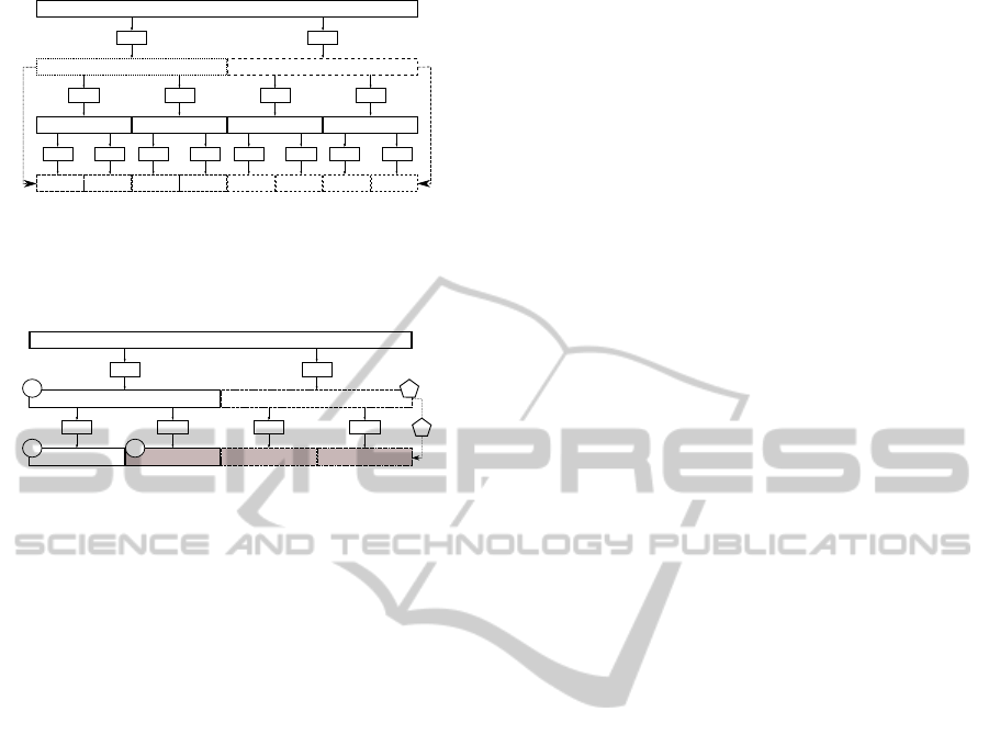
W
0,0
j=0
j=1
j=2
j=3
h
g
W
3,4
W
3,5
W
2,2
h
g
W
3,6
W
3,7
W
2,3
h
g
W
3,0
W
3,1
W
2,0
h
g
W
3,2
W
3,3
W
2,1
0
1/81/16 3/8
1/4
3/16 7/165/16 1/2
W
1,0
h
g
W
1,1
h
g
h
g
0
1/8 3/8
1/4
1/2
0
1/4
1/2
0
1/2
Figure 1: MODWPT decomposition tree showing an ex-
ample of node relocation for lower (f
l
) and upper ( f
u
) fre-
quency nodes. W
0,0
represents the original signal, f(t).
W
0,0
j=0
j=1
j=2
W
2,2
W
2,3
W
2,0
W
2,1
W
1,0
h
g
W
1,1
h
g
h
g
0
1/4 3/4
1/2
1
0
1/2
1
0
1
1
2 3
1
2
Figure 2: Search procedure for the nodes that cover the band
[0.26,0.99] Hz.
search path for this node is shown with circles. We
still have to find the node corresponding to the upper
frequency f
u
= 0.99Hz. For this frequency, (1,1) ver-
ifies equations 11 and 12. Therefore our search ends.
In Figure 2 the search path for this node is represented
with the pentagon number 1.
However, the nodes corresponding with f
l
and f
u
are at different levels of the decomposition tree: lev-
els 2 and 1, respectively. Before we can apply Equa-
tion 14, the node corresponding with f
u
, (1,1), must
be further decomposed until it reaches level 2 of the
tree, where the node corresponding with f
l
, (2, 1), is
located. In Figure 2 the relocation is represented by
pentagon number 2. Finally, the power of the band
can be computed as P([0.26,0.99]) ≈
∑
3
n=1
kW
2,n
k
2
.
3 SOFTWARE DESCRIPTION
A more detailed description on how the open source
RHRV package works can be found in (Rodr´ıguez-
Li˜nares et al., 2010). Here we will focus the descrip-
tion on the new functionality related to the extension
presented in this article.
Listing 4 shows a basic example of RHRV us-
ing Wavelet analysis. CreateHRVData() creates a
custom data structure to store all information re-
lated to the RR series and HRV analysis. Load-
BeatAscii() loads beat positions stored in the ASCII
file “BeatPosition.beats”. WFDB (Moody and Mark,
1990) data files can also be read with the function
LoadBeatWFDB(). Next, the function BuildNIHR()
computes the instantaneous heart rate (the inverse of
the time separation between two consecutive heart
beats). Outliers and points with unacceptable phys-
iological values can be removed using FilterNIHR().
An evenly spaced heart rate series is obtained with the
InterpolateNIHR() function.
The function CalculatePowerBand() calculates
the spectrogram and the power in the ULF, VLF,
LF and HF spectral bands. Although the package
provides default values for the boundaries of these
bands, they can be overridden by the user. Default
bands are ULF: [0,0.03] Hz, VLF: [0.03,0.05] Hz,
LF: [0.05,0.15] Hz, HF: [0.15,0.4] Hz. Until now,
this analysis could only be done using Shorth Time
Fourier Transform (size and shift of the analysis win-
dow can be modified by the user). The algorithms
presented in this paper were integrated into the Calcu-
latePowerBand() function, allowing both Fourier and
Wavelet analysis to be chosen by specifying an addi-
tional parameter. The default value for this parameter
is “fourier”. The function has been modified in such
a way that it is backwards compatible. Former code
using the RHRV package will keep exactly the same
behavior in the new version of the package.
When Wavelet analysis is selected in the Cal-
culatePowerBand() function, the mother wavelet to
be used in the analysis, the limits of the ULF,
VLF, LF and HF bands and the error for each of
the band boundaries can be specified by the user.
The most used mother wavelets are available: Haar
(“haar”), Daubechies (“d4”, “d6”, “d8” and “d16”)
and the least asymmetric(“la8”, “la16” and “la20”),
among others. The default mother wavelet is “d4”
(Daubechies, 2006).When Wavelet analysis is used in
the CalculatePowerBand() function, a tolerance for
the bands’ boundaries is requiered for the power spec-
trum calculations. This tolerance is is specified with
the parameter bandtolerance, which takes a default
value of 0.01.
4 RESULTS
In order to show how (at least in certain scenarios)
the HRV analysis based on the Wavelet transform pro-
vides more temporal resolution than the Fourier trans-
form, we will use a simulated RR series containing
a sharp transition in its spectral components. The
Integral Pulse Frequency Modulation (IPFM) model
(Hyndman and Mohn, 1973) has been suggested as a
functional description of the sino-atrial node. IPFM
models how the pacemaker heart cells collect electric
charge until the stored charge reaches a certain thresh-
AN OPEN SOURCE TOOL FOR HEART RATE VARIABILITY WAVELET-BASED SPECTRAL ANALYSIS
209
Listing 1: Wavelet-based analysis in RHRV.
md
=
CreateHRVData
( )
md
=
LoadBeatAscii
(
md
, ” B e a t P o s i t i o n s . beats ” )
md
=
BuildNIHR
(
md
)
md
=
FilterNIHR
(
md
)
md
=
InterpolateNIHR
(
md
,
freqhr
= 4)
md
=
CreateFreqAnalysis
(
md
)
md
=
CalculatePowerBand
(
md
,
indexFreqAnalysis
←֓
=1 ,
ULFmin
= 0 ,
ULFmax
=0.0 3 ,
VLFmin
= ←֓
0.03 ,
VLFmax
= 0.05 ,
LFmin
= 0.05 ,
LFmax
=←֓
0.15 ,
HFmin
= 0.15 ,
nHFmax
=0.4 ,
type
=”←֓
wavelet ” ,
wavelet
=”d4” ,
bandtolerance
←֓
=0.0 1)
PlotPowerBand
(
md
,
indexFreqAnalysis
=1)
old. Then the heartbeat is triggered.
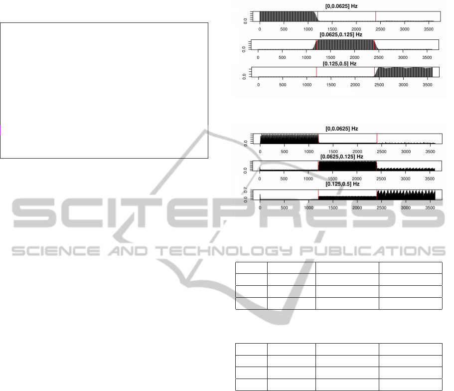
Using the IPFM model we simulated an RR time
series such us it only has spectral power in 0.03125
Hz from t = 600 s to t = 1200 s; in 0.09375 Hz
from t = 1200 s to t = 2400 s; in 0.15625 Hz from
t = 2400 s to t = 3600 s. There it should present
sharp transitions in the spectral components. We an-
alyzed the spectrum of the resulting RR series with
RHRV using Fourier (see Figure 3) and Wavelet (see
Figure 4) transforms. Frequency bands for both anal-
ysis were VLF: [0,0.0625], .LF: [0.0625,0.125] HF:
[0.125, 0.5]. The mother Wavelet used in the analysis
was Daubechies 4. Fourier analysis used a 30-second
window with 12-second shift.
In Figures 3 and 4 red vertical lines delimit each
of the three zones with different spectral components
imposed by m(t). It can be seen that wavelet analy-
sis presents better time resolution than Fourier analy-
sis. For each of the three spectral bands, and for each
of the three zones with different spectral components,
we calculated the ratio of the power that the band
presents in each zone divided by the overall power
of the band in the three zones. Theoretically, all the
power in the VLF band should be in the first zone,
all the power in the LF band should be in the second
zone, and all the power in the HF band should be in
the third zone. Therefore, the ideal ratios if perfect
frequency discrimination is obtained are (1, 0, 0), (0,
1, 0) and (0, 0, 1). Tables 1 and 2 show the real ra-
tios for Fourier and Wavelet analysis, respectively. It
can be appreciated how Fourier has better frequency
discrimination than Wavelets.
Finally, we analyzed the spectral components of
an ECG recording of an obese 54-year old male who
suffers from sleep apnea-hypopnea syndrome. The
ECG recording was performed during a sleep test.
The recording was analyzed using RHRV with the
mother Wavelet Haar and with a tolerance in the
band location of 0.01. Visual inspection of the re-
sults clearly shows that the spectral power in the band
normalized power
time(s)
Figure 3: Fourier HRV analysis of the simulated RR series.
normalized power
time(s)
Figure 4: Wavelet HRV analysis of the simulated RR series.
Table 1: Relative power for Fourier analysis.
[0,1200] [1200,2400] [2400,3600]
ULF 0,9785 0,0062 0,0153
VLF 0,0215 0,9317 0,0468
LF 0,0003 0,0030 0,9967
Table 2: Relative power for Wavelet analysis.
[0,1200] [1200,2400] [2400,3600]
ULF 0,9309 0,0456 0,0235
VLF 0,0674 0,7695 0,1631
LF 0,0087 0,3057 0,6856
[0.125, 0.250] is higher during episodes of apnea and
lower during normal breathing (see Figure 5). It
should be noted that the higher power regions are re-
marcably well localized in time. We tried to replicate
these results using Fourier, but we fail due to its lower
temporal resolution.
5 DISCUSSION AND
CONCLUSIONS
This paper presents what we believe to be the first
HRV analysis toolkit that supports Wavelet-based
spectral analysis of the RR time series. To perform
such analysis the user only has to specify the spectral
bands to be analyzed and, optionally, a tolerance for
the position of the bands’ boundaries (default toler-
ance is 0.01) and a mother Wavelet to be used in the
analysis (by default is “db4”). This functionality has
BIOSIGNALS 2012 - International Conference on Bio-inspired Systems and Signal Processing
210
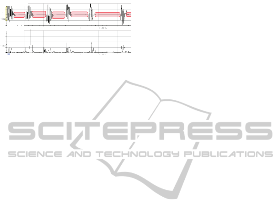
Spectralpower
Respiratoryairflow
Figure 5: Spectral power in the band [0.125, 0.250] is
higher during apnea episodes than during normal breathing.
been implemented as an extension to the open source
R package RHRV. The API of the new version of the
package is fully backwards compatible.
The results presented here suggest that Wavelet-
based analysis has a higher temporal resolution than
Fourier-based analysis. On the other hand, Fourier is
able to discriminate more precisely the spectral com-
ponents present in the signal. The results presented in
this paper are consistent with other similar tests con-
ducted by the authors.
However, it should be noted that as we descend
to lower levels in the frequency decomposition tree
when looking for a suitable node cover for a fre-
quency band, frequency resolution increases and tem-
poral resolution decreases because of the Gabor-
Heisenberg uncertainty principle for signals: (∆t∆f ≥
1/2) (Gabor, 1953). To obtain optimal temporal res-
olution, we should avoid descending to deep levels of
the tree. Our initial tests suggest that no more than
five or six levels of the frequency decomposition tree
should be expanded. In this sense, a careful selection
of the frequency bands to be analyzed provides some
control over the depth of the tree.
A corollary of the phenomenon described in the
previous paragraph is that in order to achieve optimal
temporal resolution the spectral bands used in HRV
analysis with Wavelets will probably have to differ
from those traditionally associated with ULF, VLF,
LF and HF. This opens the question of what may be
the pathophysiological significance of spectral bands
different from those which have already been widely
studied in the literature.
The mother Wavelet used in analysis also in-
fluences frequency-time resolution because it deter-
mines the filter shape. Further study on how the
mother Wavelet influences the results of the analysis
is required to understand more precisely the tradeoffs
of using Wavelets versus Fourier. For example, our
initial tests suggest that Haar Wavelet has greater time
resolution than Daubechies 4 Wavelet for HRV anal-
ysis, whereas the latter has a better filtering behaviour
than the first one.
ACKNOWLEDGEMENTS
This work was partially supported by the Spanish
MEC and the European FEDER under the grant
TIN2009-14372-C03-03, and by the Xunta de Gali-
cia under the grant PGIDIT06SIN30501PR.
REFERENCES
Akselrod, S., Gordon, D., Ubel, F., Shannon, D., Berger,
A., and Cohen, R. (1981). Power spectrum analysis of
heart rate fluctuation: a quantitative probe of beat-to-
beat cardiovascular control. Science, 213(4504):220.
Daubechies, I. (2006). Ten lectures on wavelets. Society for
industrial and applied mathematics.
Gabor, D. (1953). Communication theory and physics.
Information Theory, IRE Professional Group on,
1(1):48–59.
Hyndman, B. and Mohn, R. (1973). A pulse modulator
model for pacemaker activity. In Digest of the 10th
Int. Conf. Med. & Biol. Eng, page 223.
Kubios (2011). http://kubios.uku.fi.
Mallat, S. (1989). A theory for multiresolution signal de-
composition: The wavelet representation. Pattern
Analysis and Machine Intelligence, IEEE Transac-
tions on, 11(7):674–693.
Mallat, S. (1999). A wavelet tour of signal processing. Sec-
ond Edition. Academic Pr.
Matlab (2011). http://www.mathworks.com/index.html.
Moody, G. and Mark, R. (1990). The MIT-BIH arrhythmia
database on cd-rom and software for use with it. In
Computers in Cardiology, pages 185–188.
Nevrokard-aHRV (2011). http://www.nevrokard.eu.
Percival, D. and Walden, A. (2006). Wavelet methods for
time series analysis, volume 4. Cambridge Univ Pr.
Rodr´ıguez-Li˜nares, L., M´endez, A., Lado, M., Olivieri,
D., Vila, X., and G´omez-Conde, I. (2010). An open
source tool for heart rate variability spectral analysis.
Computer Methods and Programs in Biomedicine.
AN OPEN SOURCE TOOL FOR HEART RATE VARIABILITY WAVELET-BASED SPECTRAL ANALYSIS
211
