
SOLVING THE THREE-POINT CAMERA POSE PROBLEM IN THE
VICINITY OF THE DANGER CYLINDER
Michael Q. Rieck
Mathematics and Computer Science Department, Drake University, Des Moines, IA 50310, U.S.A.
Keywords:
P3P: Perspective, Pose, Camera, Tracking, Danger Cylinder, Trigonometry, Solid Geometry.
Abstract:
A new theorem in solid geometry is introduced and shown to be quite useful for solving the Perspective 3-Point
Pose Problem (P3P) in the general vicinity of the danger cylinder. Also resulting from this is a criterion for
partially deciding which mathematical solution is the correct physical solution. Simulations have demonstrated
the greater accuracy of the new method for solving P3P, over a standard classical method, under the following
condition. The distance from the camera’s optical center to the axis of the danger cylinder must be sufficiently
small, compared with the distance from the optical center to the plane containing the control points.
1 INTRODUCTION
1.1 Overview of P3P
The Perspective Three-Point Pose Problem (P3P) is
an old problem having its origins in photography, and
in fact is nearly as old as photography. In more recent
years, it has become a cornerstone problem in the area
of camera tracking for robotics and virtual/augmented
reality. For brevity, this problem will be referred to
simply as the “3-Point Pose Problem.”
The idea behind P3P is that a camera is positioned
at some unknown location in space and has some un-
known orientation. Three “control points” are seen
in the image produced by the camera. The positions
of these points in physical space are presumed to be
known in advance. Camera intrinsic values, in partic-
ular the focal length, are also presumed to be available
for computations. The goal of course is to determine
the position and orientation of the camera. In this re-
port, we will restrict attention to only finding the cam-
era’s position in space. From here it is not particularly
difficult to also determine its orientation.
Established methods for solving P3P generally run
into difficulty when the camera’s optical center (the
point at which the lines-of-sight intersect) is too close
to the so-called “danger cylinder” region. A number
of studies of this phenomenon have been made. Sev-
eral of these are mentioned in Subsection 1.2. It has
been observed that repeated solutions occur when the
optical center is on the danger cylinder.
1.2 Related Work
Since it was first introduced and solved (Grunert,
1841), various efforts have been made to better un-
derstand P3P and its underlying system of equations.
Alternative methods for solving P3P have also been
introduced, though often these either essentially pro-
ceeded along similar lines as the original solution,
or else required complicated numerical analysis tech-
niques.
Some of the mid-twentieth century work, much of
it motivated by aerial reconnaissance concerns, can
be found in (Merritt, 1949), (M
¨
uller, 1925), (Smith,
1965) and (Thompson, 1966). (Haralick et al., 1994)
provides an excellent extensive survey of the state of
P3P at the end of the twentieth century.
Several recent studies have classified solutions,
such as (Faug
`
ere et al., 2008), (Gao et al., 2003),
(Sun and Wang, 2010), (Tang et al., 2008), (Tang
and Liu, 2009), (Wolfe et al., 1991), (Zhang and
Hu, 2005). Some of the more recent algorithms for
solving P3P, and generalizations and restrictions of
it, can be found in (DeMenthon and Davis, 1992),
(Nist
´
er, 2007), (Pisinger and Hanning, 2007), (Rieck,
2010), (Rieck, 2011), (Xiaoshan and Hangfei, 2001).
A recent reexamination of the danger cylinder phe-
nomenon can be found in (Zhang and Hu, 2006).
1.3 Layout of this Report
Section 2 of this report introduces a curious new theo-
rem in solid geometry, intimately related to P3P. Sec-
335
Q. Rieck M..
SOLVING THE THREE-POINT CAMERA POSE PROBLEM IN THE VICINITY OF THE DANGER CYLINDER.
DOI: 10.5220/0003725403350340
In Proceedings of the International Conference on Computer Vision Theory and Applications (VISAPP-2012), pages 335-340
ISBN: 978-989-8565-04-4
Copyright
c
2012 SCITEPRESS (Science and Technology Publications, Lda.)

Figure 1: Danger cylinder (top-down view).
tion 3 explains how this theorem can serve as the ba-
sis of a new approach to solving P3P in the vicinity
of the danger cylinder. Subsection 3.1 takes a closer
look at the special case where the control points are
equidistant from one another. Subsection 3.2 explains
how the new approach for solving P3P can be refined,
by applying the Newton-Raphson method. Subsec-
tion 3.3 explores the long-standing and thorny issue
of choosing the correct P3P solution from among the
several possible mathematical solutions.
2 ANALYSIS
2.1 Preliminaries
Let us now begin a careful examination of P3P. When
the three control points are not collinear, they lie on
a unique circle, which is a basic fact from classical
geometry. We will assume henceforth that the con-
trol points are not collinear, and to simplify the no-
tation, will suppose that the unit of distance used is
such that this circle has radius one. The formulas to
be presented in this report can easily be scaled so as
to accommodate an arbitrary radius. (In Theorem 1,
just divide d
1
,d
2
,x,y and z by this radius.)
A Cartesian coordinate system will be set such
that the three control points, P
1
, P
2
, P
3
, lie on the unit
circle centered about the origin, in the xy-plane. For
j = 1,2,3, let (cos φ
j
,sinφ
j
,0) be the coordinates of
P
j
, with −π ≤ φ
j
≤ π, and let t
j
= tan(φ
j
/2). Also
let d
j
be the distance between the two control points
other than P
j
. From the standpoint of P3P, all these
quantities are known a priori. The unknown coordi-
nates of the camera’s optical center P will simply be
denoted (x,y,z). Let r
j
be the distances between P
and P
j
( j = 1,2,3). For j = 1,2,3, let θ
j
be the angle
at P created by the two rays to the two control points
other than P
j
. Let c
j
= cos θ
j
. These angles and their
cosines are presumed to be known since they are eas-
ily computed from the control point images and cam-
era intrinsics.
The “danger cylinder” is the circular cylinder that
contains the three control points, and whose axis is
perpendicular to the plane containing these control
points. With the setup described here, the danger
cylinder is given by the equation x
2
+ y
2
= 1. It
is a well-studied fact that when the optical center is
on or near the danger cylinder, traditional techniques
for solving the 3-Point Pose Problem run into diffi-
culties caused by imprecision in numerical computa-
tions. Figure 1 shows the situation when the optical
center is on the danger cylinder, and above the plane
containing the control points.
A number of identities need to be established,
and there is not enough room to report them here.
They follow quickly from standard trigonometric
identities. An important consequence of these facts
for the analysis of P3P to be presented, is as follows.
Lemma 1. The quantities r
2
1
, r
2
2
, r
2
3
, d
2
1
, d
2
2
, d
2
3
, c
2
1
,
c
2
2
, c
2
3
and c
1
c
2
c
3
can all be expressed as rational
functions of t
1
, t
2
, t
3
, x, y and z.
Now, in the 3-Point Pose Problem, it is supposed
that the quantities c
1
,c
2
,c
3
,d
1
,d
2
and d
3
are known,
and that the goal is to determine the optical center co-
ordinates x, y and z. We are of course assuming that
θ
1
,θ
2
,θ
3
,φ
1
,φ
2
,φ
3
,t
1
,t
2
and t
3
are known too, but not
r
1
,r
2
and r
3
.
The classical approach involves using the Law of
Cosines to establish three quadratic equations in the
unknowns r
1
,r
2
,r
3
, or related quantities. One then
eliminates two of the unknowns, producing a polyno-
mial equation in the remaining unknown. After ob-
taining the roots of this polynomial, it is still neces-
sary to decide which root is the correct one.
Assuming that the correct solution is chosen, it is
straightforward to then determine x, y and z. This ap-
proach works fairly well, as long as the control points
are reasonably far apart, the optical center is reason-
ably close to the control points and the optical center
is reasonably far from the danger cylinder. The ex-
act meaning of these conditions depends of course on
the precision used in performing floating point com-
putations. In practice, camera pixelation also causes
imprecision that can adversely affect the results.
2.2 The Quantity η
An important quantity that can be computed based
solely on the (known) cosines c
1
, c
2
and c
3
is
η =
q
1 −c
2
1
−c
2
2
−c
2
3
+ 2c
1
c
2
c
3
.
VISAPP 2012 - International Conference on Computer Vision Theory and Applications
336

By Corollary 1, we see that η
2
can be expressed as a
rational function of t
1
, t
2
, t
3
, x, y and z.
Lemma 2. r
1
r
2
r
3
η equals six times the volume of
the tetrahedron whose vertices are the optical center
and the three control points. This also equals the
volume of the parallelepiped having these four points
among its vertices, with each control point adjacent to
the optical center along an edge of the parallelepiped.
Henceforth, we will suppose that the control points
and the optical center are not coplanar, so that η > 0.
2.3 A Useful Quadratic Polynomial
Before stating and proving the main theorem (Theo-
rem 1) of this report, it will be helpful to introduce the
following function of x and y, for a given angle φ:
Σ(φ;x,y) = (sin φ)(y
2
−x
2
) +(cos φ)(2xy)
= (sin φ) [−ρ
2
cos(2θ)] +(cos φ)[ρ
2
sin(2θ)]
= ρ
2
sin(2θ −φ) ,
where (x,y) = (ρ cos θ, ρ sin θ). As a function of x and
y, this is a homogeneous quadratic polynomial having
a saddle point at the origin. It is clearly symmetric
about the origin too. This function will play an inter-
esting role in Theorem 1.
2.4 A New Theorem in Solid Geometry
In this subsection, the essential theorem of this report
will be stated. The theorem relates a simple rational
function of the known cosines c
1
, c
2
and c
3
, and the
known separation distances d
1
and d
2
, to a two-part
rational function of the unknowns x, y, z. The second
part of this latter function vanishes on the danger
cylinder x
2
+ y
2
= 1, and also diminishes in signifi-
cance when z
2
grows large relative to |x
2
+ y
2
−1|.
The other (first) part is particularly simple, essentially
being just the Σ function shifted and scaled.
Theorem 1.
d
2
1
(1 −c
2
2
) −d
2
2
(1 −c
2
1
)
η
2
=
A(φ
1
,φ
2
,φ
3
; x,y) +
B(φ
1
,φ
2
,φ
3
; x,y)
1 −x
2
−y
2
z
2
,
where
A(φ
1
,φ
2
,φ
3
; x,y) = csc
φ
1
−φ
2
2
·
Σ
φ
1
+ φ
2
+ 2φ
3
2
; x + cos φ
3
, y + sin φ
3
and
B(φ
1
,φ
2
,φ
3
; x,y) =
d
2
1
−d
2
2
4
−
csc
φ
1
−φ
2
2
Σ
φ
1
+ φ
2
+ 2φ
3
2
;
x −
cosφ
1
+ cosφ
2
2
, y −
sinφ
1
+ sinφ
2
2
.
The above remains true when the subscripts 1, 2 and
3 are permuted.
3 APPLICATION TO P3P
We now turn our attention to leveraging Theorem 1
in order to obtain a practical and successful method
for rapidly and accurately estimating a solution to the
3-Point Pose Problem, on or near the danger cylinder.
Corollary 1. Assuming that d
1
, d
2
, d
3
, c
1
, c
2
and c
3
are known, and assuming that |x
2
+ y
2
−1|/z
2
is suf-
ficiently small, the unknowns x and y approximately
satisfy a pair of independent quadratic polynomials.
By eliminating one of the unknowns, the result is a
polynomial in the other unknown, of degree four.
Once x and y have been estimated, z can be esti-
mated by means of Fact 7 in Subsection 3.2 of (Rieck,
2011). u there is z
2
here. Essentially, it is shown there
that
(1 +t
2
1
)(1 +t
2
2
)(1 +t
2
3
) c
1
c
2
c
3
−
(1 +t
1
t
2
)(1 +t
2
t
3
)(1 +t
3
t
1
) ] / η
2
equals a quadratic polynomial in z
2
, with coefficients
that are rational functions of t
1
, t
2
, t
3
, x, y, plus a quan-
tity that factors as (x
2
+ y
2
−1)/z
2
times another ra-
tional function of t
1
, t
2
, t
3
, x, y.
3.1 Special Case
In the special case where φ
1
= 2π/3, φ
2
= −2π/3 and
φ
3
= 0 (so that t
1
=
√
3, t
2
= −
√
3 and t
3
= 0), the
control points form the vertices of an equilateral trian-
gle, with d
1
= d
2
= d
3
=
√
3. A preliminary analysis
of this special case appears in (Rieck, 2010). The for-
mulas in Theorem 1 (of the current report) now take
on particularly simple forms, as follows.
SOLVING THE THREE-POINT CAMERA POSE PROBLEM IN THE VICINITY OF THE DANGER CYLINDER
337
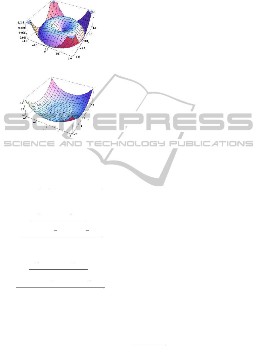
Figure 2: Errors when z = 5 (narrow view).
Figure 3: Errors when z = 5 (wider view).
Corollary 2. When φ
1
= 2π/3, φ
2
= −2π/3 and φ
3
=
0, we have the following three equations:
(c
2
1
−c
2
2
) / η
2
=
4(1 +x)y
3
+
2(x
2
+ y
2
−1)(1 + 2x)y
3 z
2
,
(c
2
2
−c
2
3
) / η
2
=
(
√
3x + y)(x −
√
3y −2)
3
+
(x
2
+ y
2
−1)(
√
3x + y)(x −
√
3y −1)
3 z
2
,
(c
2
3
−c
2
1
) / η
2
=
(
√
3x −y)(−x −
√
3y +2)
3
+
(x
2
+ y
2
−1)(
√
3x −y)(−x −
√
3y +1)
3 z
2
.
Of course these are not independent. The right-
hand sides sum to zero, as clearly do the left-hand
sides. When the quantity (x
2
+ y
2
−1)/z
2
is suffi-
ciently small that the second terms of the right-hand
sides can be ignored, for approximation purposes, the
first equation can immediately be solved for y. This
can then be substituted into either of the other two
equations to obtain a quartic equation in x.
Mathematica
R
simulations were conducted using
this method.
1
With z = 5, the errors that resulted
in estimating (x,y,z) are shown in Figures 2 and 3.
The error metric used here is simply the Euclidean
distance between the estimated optical center and the
actual optical center (x, y,z). Figure 2 shows impres-
sive results when x
2
+ y
2
≤ 1. We see in Figure 3
that the errors become much more significant when
1 < x
2
+ y
2
≤ 2. Notice the difference in error scales
between Figures 2 and 3. Also, for greater values of
z, but keeping say x
2
+y
2
≤2, the errors become con-
siderably smaller.
3.2 Refinement
Once an approximate solution to the 3-Point Pose
Problem has been obtained, numerical methods can
be applied to improve it. This can be done for the gen-
eral problem, but attention here will be limited here to
the special case where the control points are equally
spaced. One of several ways to proceed is to sim-
ply take the three Corollary 2 equations, and apply a
multivariate version of the Newton-Raphson method
to the resulting system of equations.
However, another approach which has proven to
be highly successful, is considerably simpler. Starting
with the same basic equations, for each, subtract from
both sides the term that includes the division by z
2
(i.e.
the last term). The resulting left side of the equation is
then computed using the known values for the c
j
, d
j
and η, and using the already estimated values for x, y
and z. However, the x, y and z on the right side of the
equations are treated as unknowns to be determined.
Similar to before, the equations that result from
this approach can be manipulated to produce a quar-
tic equation in x. The already estimated value for x is
then used as an initial value for a single iteration of
the Newton-Raphson method on this polynomial in
order to obtain a better estimate for x. From this, bet-
ter estimates are then obtained for y and z. The whole
process can be repeated as desired.
Prior to applying the refinement method though,
for technical reasons, it is prudent to first determines
which of the three control points is nearest to the pro-
jection of the estimated optical center onto the xy-
plane. One can then effectively rotate the setup math-
ematically so that this control point takes the place of
the control point at (1,0,0). This improves the results.
Figure 4 shows the vast improvement that results
from applying four iterations of this refinement tech-
nique to the initial estimate for (x,y,z). Note the con-
trast in the error scale between Figures 3 and 4. Out to
1
A Mathematica notebook for the results in this report is
available from the author upon request.
VISAPP 2012 - International Conference on Computer Vision Theory and Applications
338

Figure 4: Errors after four refinement iterations.
a radius of two (in the xy-plane projection), the errors
are now typically well below 0.005.
3.3 Solution Selection
In the above simulations, the real-valued mathemati-
cal solutions were ordered, based on increasing values
of x
2
+ y
2
. Assuming the optical center is fairly close
to the danger cylinder, a simple-minded strategy for
trying to decide which solution is the correct one, is
to simply use the first solution, that is, the one with
the least value of x
2
+ y
2
. This simple minded strat-
egy chooses the correct solution anytime the optical
center is inside the danger cylinder. However, it is
generally not reliable when the optical center is out-
side the danger cylinder.
An interesting curve that arises in analyzing the
mathematical solutions is the “deltoid” (also called a
“tricuspoid” or “Steiner curve”) seen in Figure 5, and
given by the quartic equation
2x
2
y
2
+x
4
+y
4
−8x
3
+24xy
2
+18x
2
+18y
2
−27 = 0.
Interpreting this equation in three dimensions
yields a “deltoidal cylinder.” When the optical cen-
ter is outside this deltoidal cylinder, there are almost
always at most two real-valued mathematical solu-
tions. In this case, the first solution (based on the
x
2
+ y
2
-ordering) tends to be the correct solution, as
long as the optical center is not too far from the del-
toidal cylinder, nor its projection onto the xy-plane too
close to a control point.
In contrast, assuming |z| is not too small, when the
optical center is inside the deltoidal cylinder, there al-
most always seem to be four real-valued mathemati-
cal solutions, all inside this region, with exactly one
of these being inside the danger cylinder. The correct
solution tends to be among the first two solutions. As
already indicated, if the optical center is inside the
danger cylinder, then the first solution will always be
correct.
If there were a practical way to know whether the
optical center was inside or outside the danger cylin-
Figure 5: Deltoid (and dashed unit circle).
der, then this could be used to achieve solution esti-
mates with average error values close to those seen
in Figure 4. Note that that figure was based on using
the techniques developed in Subsections 3.1 and 3.2,
but then always selecting the best of the mathematical
solutions produced.
4 CONCLUSIONS
A new theorem in solid geometry has been intro-
duced. When applied to the 3-Point Pose Problem,
this theorem gives a surprising connection between
the unknown position of the camera’s optical center
and known data. This known data consists simply of
the distances between the control points, and also the
cosines of certain angles that can be determined from
the images of the control points in the image plane of
the camera.
This theorem is particularly useful when the opti-
cal center is on or at least somewhat close to the dan-
ger cylinder region, as compared with the distances
from the optical center to the control points. When
on the danger cylinder, it can be efficiently and ac-
curately applied to directly determine the position of
the optical center. When only near the danger cylin-
der, it can be used to reasonably estimate this position.
Straightforward applications of Newton-Raphson can
then dramatically improve this estimated position.
Criteria for selecting the correct physical solution
from among as many as four real-valued mathemat-
ical solutions were also explored. This proved to be
success whenever the optical center was located in-
side the danger cylinder, and often when it was out-
side but not too far from the danger cylinder.
Figure 6 shows the results of simulations using
single-precision C++ code.
2
The simulations demon-
strate the greater accuracy of the approach devel-
oped in this report (“DSA-based”), against a classical
2
C++ source code is available from the author upon re-
quest.
SOLVING THE THREE-POINT CAMERA POSE PROBLEM IN THE VICINITY OF THE DANGER CYLINDER
339

Figure 6: C++ simulation using single precision.
method (Grunert, 1841). The danger cylinder radius
in the simulation was 0.17 meters, and the horizon-
tal axis of the graph in Figure 6 reflects the distance
from the optical center to the danger cylinder axis.
The vertical axis of the graph shows the average er-
ror, as a distance in meters between the actual optical
center and the position computed by the method.
The new method was also much more consis-
tent, while Grunert’s method sometimes produced
very inaccurate results. Grunert’s method occasion-
ally showed an error distance that was a large fraction
(about a half) of the distance between the optical cen-
ter and the control points. The new method, by con-
trast, was never off by more than five or six percent.
REFERENCES
DeMenthon, D. and Davis, L. S. (1992). Exact and approx-
imate solutions of the perspective-three-point prob-
lem. IEEE Trans. Pattern Analysis and Machine In-
telligence, 14(11):1100–1105.
Faug
`
ere, J.-C., Moroz, G., Rouillier, F., and El-Din, M. S.
(2008). Classification of the perspective-three-point
problem, discriminant variety and real solving poly-
nomial systems of inequalities. In ISSAC’08, 21st Int.
Symp. Symbolic and Algebraic Computation, pages
79–86. ACM.
Gao, X.-S., Hou, X.-R., Tang, J., and Cheng, H.-F. (2003).
Complete solution classification for the perspective-
three-point problem. IEEE Trans. Pattern Analysis
and Machine Intelligence, 25(8):930–943.
Grunert, J. A. (1841). Das pothenotische problem in er-
weiterter gestalt nebst
¨
uber seine anwendungen in der
geod
¨
asie. In Grunerts Archiv f
¨
ur Mathematik und
Physik, volume 1, pages 238–248.
Haralick, R. M., Lee, C.-N., Ottenberg, K., and N
¨
olle, N.
(1994). Review and analysis of solutions of the three
point perspective pose estimation problem. J. Com-
puter Vision, 13(3):331–356.
Merritt, E. L. (1949). Explicit three-point resection in space.
Photogrammetric Engineering, 15(4):649–655.
M
¨
uller, F. J. (1925). Direkte (exakte) l
¨
osung des einfachen
r
¨
uckw
¨
artsein-schneidens im raume. In Allegemaine
Vermessungs-Nachrichten.
Nist
´
er, D. (2007). A minimal solution to the generalized
3-point pose problem. J. Mathematical Imaging and
Vision, 27(1):67–79.
Pisinger, G. and Hanning, T. (2007). Closed form monoc-
ular re-projection pose estimation. In ISIP ’07, IEEE
Int. Conf. Image Processing, volume 5, pages 197–
200.
Rieck, M. Q. (2010). Handling repeated solutions to the
perspective three-point pose problem. In VISAPP ’10,
Int. Conf. Computer Vision Theory and Appl., pages
395–399.
Rieck, M. Q. (2011). An algorithm for finding repeated
solutions to the general perspective three-point pose
problem. J. Mathematical Imaging and Vision. DOI:
10.1007/s10851-011-0278-y (to appear in print).
Smith, A. D. N. (1965). The explicit solution of the single
picture resolution problem, with a least squares adjust-
ment to redundant control. Photogrammetric Record,
5(26):113–122.
Sun, F.-M. and Wang, B. (2010). The solution distribu-
tion analysis of the p3p problem. In SMC ’10, Int.
Conf. Systems, Man and Cybernetics, pages 2033–
2036. IEEE.
Tang, J., Chen, W., and Wang, J. (2008). A study on the
p3p problem. In ICIC ’08, 4th Int. Conf. Intelligent
Computing, volume 5226, pages 422–429.
Tang, J. and Liu, N. (2009). The unique solution for p3p
problem. In SIGAPP ’09, ACM Symp. Applied Com-
puting, pages 1138–1139. ACM.
Thompson, E. H. (1966). Space resection: failure cases.
Photogrammetric Record, 5(27):201–204.
Wolfe, W. J., Mathis, D., Sklair, C. W., and Magee, M.
(1991). The perspective view of three points. IEEE
Trans. Pattern Analysis and Machine Intelligence,
13(1):66–73.
Xiaoshan, G. and Hangfei, C. (2001). New algorithms for
the perspective-three-point problem. J. Comput. Sci.
& Tech., 16(3):194–207.
Zhang, C.-X. and Hu, Z.-Y. (2005). A general sufficient
condition of four positive solutions of the p3p prob-
lem. J. Comput. Sci. & Technol., 20(6):836–842.
Zhang, C.-X. and Hu, Z.-Y. (2006). Why is the danger
cylinder dangerous in the p3p problem? Acta Auto-
matica Sinica, 32(4):504–511.
VISAPP 2012 - International Conference on Computer Vision Theory and Applications
340
