A STRATEGIC SIMULATION TOOL FOR CAPABILITY-BASED

JOINT FORCE STRUCTURE ANALYSIS

Cheryl Eisler and Dave Allen

Centre for Operational Research and Analysis, Defence R&D Canada, 101 Colonel By Drive, Ottawa, Canada

Keywords: Discrete Event Simulation, Monte Carlo, Force Structure Analysis, Fleet Mix, Capability-Based Planning.

Abstract: This paper describes a stochastic discrete event simulation model for scheduling of joint military force

structures. The model employs capability-based methods to link scenario requirements to force structure

assets. Assignment of assets to scenarios is designed to attempt to mimic the decisions of a military

scheduler. Force structure performance is evaluated based on how well and how often scenario capability

requirements are met. The model output permits options analysis, capability gap analysis, determination of

optimal force structure composition, and evaluation of force structure performance in the face of changing

requirements and policies (such as readiness and sustainment, operations tempo, and personnel tempo

constraints).

1 INTRODUCTION

Determining the size and composition of a future

military force structure

is a problem that can be

approached from many different directions, and is

often driven by nation-specific policies, processes,

and objectives. It is also a question of the depth and

breadth of exploration required; depth in terms of

the level of fidelity that is used to model the force

structure, and breadth across military services.

In practice, quantitative evaluation of force

structures range from “back-of-the-envelope” type

calculations (e.g., with two bases, two ships are

required at each so that one is always available when

one is in maintenance) or subject matter expert

(SME) opinion, to detailed theatre level combat

modelling (e.g., Bulut, 2001, Gallagher and Kelly,

1991) or campaign analysis (Taylor and Lane,

2004). Low fidelity models are easy to generate, but

tend to rely on broad-ranging assumptions and are

subject to significant criticism regarding objectivity.

Ideally, high fidelity models would be used to

determine the performance of the total force against

high-fidelity models are very data intensive and/or

use physics-based approaches that are time-various

threats across multiple scenarios (Farr et al., 1994).

While they are significantly less subjective,

consuming to evaluate and difficult to extrapolate

for future capability. Taking a moderated approach,

medium fidelity models focus on resource allocation

(how many are needed) rather than resource

effectiveness (how likely the mission can be

accomplished). This is a specialized application of

general scheduling and routing problems, for which

many customized models have been developed.

Service-specific scheduling models abound.

Logistic problems such as sealift (Salmeron et al.,

2009), airlift (Wu et al., 2009, Wesolkowski and

Billyard, 2008, Baker et al., 2002) – to name but a

few, or a combined mobility problem (Mattock et

al., 1995) are well developed, but difficult to expand

for use across services. If not focused on airlift, air

force structure models tend to be driven by

maintenance requirements and facilities (Mattila et

al., 2008). Army force structure analysis is highly

separated between personnel-driven models

(Klerman et al., 2008) and vehicle fleet mixes

(Whitacre et al., 2008, Abbass et al., 2007,

Walmsley and Hearn, 2004, Brown et al., 1991).

Naval deployment scheduling applications are

common (Zadeh, 2009, Horn et al., 2007, Dugan,

2007, and others). Five naval fleet planning

applications (Gauthier et al., 2008, Fildes, 2006,

Greer et al., 2005, Crary et al., 2002, Cortez and

“Force structure” is a term used to designate the set o

assets within a military unit and the inter-dependence

etween these assets, as well as their home base. Fo

example, a naval force structure could include all the ships

and crews, as well as the infrastructure supporting them.

Eisler, C. and Allen, D.

A STRATEGIC SIMULATION TOOL FOR CAPABILITY-BASED JOINT FORCE STRUCTURE ANALYSIS.

DOI: 10.5220/0003727800210030

In Proceedings of the 1st International Conference on Operations Research and Enterprise Systems (ICORES 2012), pages 21-30

ISBN: 978-989-8425-97-3; ISSN: 2184-4372

 2023 by His Majesty the King in Right of Canada as represented by the Minister of National Defence and SCITEPRESS – Science and Technology Publications, Lda. Under

CC license (CC BY-NC-ND 4.0)

Kaiser, 1991) exhibit properties that may be useful if

applied to joint force structure scheduling. Only two

references (Davis, 2002, Farr et al., 1994) were

found that attempt to tackle joint force structure

problems. The first leaves much of the methodology

undefined, and the second is a deterministic model

that does not optimize over a range of requirements.

Selection of a force structure must balance

strategic policies and objectives, while maintaining

realism at the operational and tactical levels – and

still provide answers in a timely fashion. To achieve

a measure of balance among these conflicting

drivers, Defence R&D Canada’s Centre for

Operational Research and Analysis (DRDC CORA)

has developed a strategic level simulation tool,

known as Tyche. Tyche takes a moderate-fidelity

approach to joint force structure analysis that utilizes

capability-based planning. The next section

describes the Tyche model, including novel features

and modelling limitations. Section 3 provides a

sample joint force structure case study. Conclusions

are given in Section 4.

2 THE SIMULATION MODEL

Tyche is a stochastic simulation model that

schedules the deployment of assets within a force

structure to address a set of missions. The

assignment of assets to missions is based on a set of

predefined rules that attempt to reproduce the

decisions made by a military scheduler. Scheduling

assignment is capability-based; meaning each

mission requires a set of capabilities for success, and

each asset type provides a set of capabilities that

may or may not overlap with the required mission

capabilities. The force structure measure of

performance (MOP) is evaluated based on how well

and how often the missions’ capability requirements

are met.

When it was originally developed in 2004, Tyche

was designed to model naval force structures. It was

later adapted to accommodate joint asset types;

however, a number of assumptions within the

program affect the range of detailed joint military

applications. These limitations will be discussed in

the following subsections, and are slated for future

development.

Tyche is divided into three interconnected

environments: a data entry environment where the

data required to perform simulations are entered; a

run environment where the specifics of the desired

simulations are entered; and a data exploration

environment where the MOP and run output can be

visualized and further investigated. The function of

these three environments is described.

2.1 Data Structure

There are five fundamental data structures employed

within the Tyche model to build a simulation:

capabilities, asset types, bases/theatres, scenarios,

and force structures.

2.1.1 Capabilities

While capabilities simply refer to any ability to

perform a task, they provide a flexible way to link

mission requirements to force structures. Most force

structure analysis models are either platform-based

(meaning requirements are defined in terms of the

number and type of platforms for mission success)

or physics-based (specifying physical characteristics,

such as dimensional capacity for air or sea lift).

Tyche is unique in that the user can define

capabilities to suit the simulation model

requirements. Typical capabilities used for military

simulations simulation include command and control

(C2), surveillance, firing, jamming, transportation,

etc. Quality and quantity factors are associated with

each capability. Quality is a scale on (0,1] for

relative comparison; quantity is a positive integer

(

∈

). This permits objective comparison of often

subjective evaluations (e.g., the higher C2 capability

of a destroyer compared to a frigate is modelled

model by a higher numerical quality), as well as

encompassing the physical characteristics in a

single, broader definition of capability (e.g., lane

meters of sea lift is associated to a numerical

quantity).

2.1.2 Asset Types

Asset types are defined to allow for modelling of

equipment, personnel, weapons, modules, etc., and

include both dynamic and static assets (static assets

cannot travel to theatre on their own, such as

maritime helicopters). Various levels of fidelity in

the modelling of assets are possible, which positions

the tool well to cross between coarse strategic-level

studies and more detailed operational-level analysis.

One limitation that the user must bear in mind when

defining asset types is the timescale within Tyche.

The smallest unit of time is one day, and simulations

are intended to run over multiple years (an

assumption that was suitable for naval applications).

A user-selectable timescale is planned for future

versions of the software to accommodate force

ICORES 2012 - 1st International Conference on Operations Research and Enterprise Systems

structures that commonly operate on smaller

timescales.

Tyche also allows for modelling of external

assets; those that could be chartered or assumed

available (based on a given probability) from

another source. This allows for simple modelling of

assets about which little knowledge is available.

The concept of “level” is introduced as a key

element in the modelling of assets. Levels are used

to model the different states or working conditions

of the assets such as the readiness states,

breakdowns, maintenance, training, and leave. In

essence, the levels allow the modelling of variations

of the capability supplied by the assets under user-

defined circumstances. An asset type’s levels are

prioritized, so that critical tasks can override (or

bump) less important tasks. Associated with each

prioritization instruction between two given levels

are a bump time, a bump penalty, and rescheduling

instructions for the bumped level.

In addition, levels are characterized by type, a set

of capability supply and demand, and the optional

inclusion of constraints with regards to the possible

asset assignment. Level types include random (e.g.,

to model unforeseen breakdowns), scheduled (e.g.,

to model maintenance periods), on-demand (e.g., to

model mission assignment), and follow-on (e.g., to

model a quality of life break following a long

mission assignment). The set of capability supply

and demand associated with the asset type is specific

to each level. For example, a user may model levels

of readiness with different degrees of capability and

response time associated with each. Synergistic

effects can also be captured; as when two assets are

assigned together to produce a higher level

capability of either alone (e.g., a helicopter

embarked on a frigate to increase the effectiveness

of the frigate’s surveillance capability).

The association of capability demand to assets

leads to the ability to model multi-layer and co-

dependent capability demand chains. An asset may

demand capability, just as a scenario would. This is

common with static assets requiring transportation

into theatre. Co-dependent demand arises when a

demanded asset requires capability supplied by the

asset requiring it. For example, a helicopter requires

transportation to theatre which can be provided by a

frigate, and in reverse the frigate requires a

helicopter to provide surveillance.

A distinction between capability supply and

capability demand is in the number of associated

attributes. Capability supplies have only an assigned

quantity and quality which specify the number and

the degree to which the capability is provided. On

the other hand, in addition to a quantity, capability

demands have two quality values specified: the

required and marginal quality levels. The required

quality determines the degree of desired quality for

satisfactory performance, and the marginal quality

provides the degree needed for minimum

performance standards. The quantity determines the

number of requested capabilities to support a single

asset type at the level being defined. In addition to

the quality and quantity, the capability demand also

requires a weight, which is used to quantify the

importance of this capability demand with regard to

other capability demands. Finally, a capability

demand can be deemed “essential”. If an essential

capability demand cannot be satisfied at the required

quality with a capability supply from another asset,

then this asset will not be able to go to this level. For

example, for a ship to leave a port, it needs to be

manned by a crew. If there is no crew available, then

the ship will stay alongside. Thus, the crew provides

a capability that is essential to the ship when it is

requested to leave the port.

Constraints on maximum or minimum duration

or on the number of occurrences of one or more

levels over a given period of time can also be

imposed to mimic scheduling limitations such as

maximum time used (e.g., annual flight hours for

aircraft), or frequency of usage in long-term high-

intensity missions to maintain personnel tempo.

2.1.3 Bases and Theatres

Bases are locations where assets are stationed when

not assigned to a mission and theatres are locations

where missions occur. Neither is given physical

coordinates, merely relative distances to one

another. No units of distance are specified, allowing

the user to determine a physical route for travel that

is compatible with the speed unit that will be

associated with the assets using these locations. For

example, two bases could be used to represent a

single location from which air and sea assets depart.

An over-land great circle arc distance would be used

for the distance that air assets travel, while an over-

water distance (often much larger, when taking into

account land mass detours) would be used for the

sea assets.

In this formulation, a simple model of one home

base for each asset, which then travels to a single

theatre for a scenario, is used. Waypoints for

intermediate activities (such as resupply), and

forward stationing of assets, are more complex

behaviours that are under consideration to better

model aspects of joint force operation.

A STRATEGIC SIMULATION TOOL FOR CAPABILITY-BASED JOINT FORCE STRUCTURE ANALYSIS

2.1.4 Scenarios

Scenarios represent missions (or a group of

missions) to which assets are assigned. A scenario is

defined in terms of phases, which represent the

variation of capability demand required over time

(e.g., pre-crisis a scenario might require more

diplomatic and economic intervention and a show of

force, while later phases may demand combat

capabilities and non-combatant evacuation). Each

scenario also has a number of possible theatres, each

having a probability of assignment. Each phase can

be independent, or linked to one or more other

phases. Consequently, activities of varying

capability demand, duration, and location can be

modelled.

In terms of associated attributes, the phases of a

scenario show many similarities with the levels of an

asset. There are three types of phases: scheduled,

random, or follow-on. As with the level, a scheduled

phase requires a start date and frequency that set the

precise dates the phase will occur. For the random

phases, only the frequency must be specified; a

Poisson distribution is used to determine the

occurrence of these scenarios (see Section 2.2.1).

The main difference between levels and phases is

the absence of the timing constraints and capability

supply for the latter, as well as the appearance of

more complex scoring criteria. The scoring criteria

determine how to select assets for the phase, by

means of a cost function for various choices of

assets and selecting the best additive score of all the

possibilities.

The cost function will be defined in

Section 2.2.2.

2.1.5 Force Structures

A force structure stores all the assets from the

different asset types that would be used for a given

simulation run, including possible external assets.

The term “fleet” was used but the assets are not

limited to naval types. Assets are defined by

specifying type, home base, and a scheduling offset.

The offset is a number that specifies the number of

days by which the start date of the scheduled levels

of the asset will be shifted with respect to other

assets of the same type. Currently, many force

structures can be defined, but each must be run

individually. The possibility of incorporating the

model inside an optimization routine is under

consideration, so as to determine the optimal force

structure to meet a set of requirements.

2.2 Simulation Procedure

At its core, Tyche is a discrete-event scheduling

program. For every iteration, the force structure data

are initialized, a list of events is generated where

each event requires assets to be assigned, and the

“best” available assets are then assigned to these

events. Data is then output in the form of an

operational schedule for each iteration. Data for

reinitializing the random number generator are also

output to allow for continuation of simulation runs at

a subsequent time (this can be useful in the event of

computer issues).

2.2.1 Event Generation

The list of events is generated at the start of every

iteration, and updated as the clock progresses in the

simulation. An event occurs every time a scenario

phase begins or an asset changes level. To build the

list of events, Tyche first selects a random date,

which is the initial date at which the simulation

starts. All scheduled events are created in relation to

this date (where day 0 is the first day of the calendar

year). Random phases and levels are determined

from a Poisson distribution with a frequency of

occurrence per year of λ. For an iteration of n years,

the number of events (N) is determined by selecting

a random number, r uniformly distributed on [0,1],

and applying Eq. (1).

()

∑

−

∑

−

≤<∈=

ereiiN

|with

(1)

Note that the sum over the integer j from 0 to i-1

is set to 0 in the case i=0. The start date of each

random event is then selected from the set of days

inside the time window using a uniform distribution.

The duration of events that cross the number of

years simulated are reduced to fit completely inside

the time window. Events that are too short to have

any assets assigned (based on minimum preparation

and travel time) are removed from the simulation.

As a result, the first and last year of all simulation

iterations are not counted in the statistics generation

(see Section 2.3.1) to eliminate this burn-in effect.

There are times during the simulation run when

the event list can be modified. While follow-on

phases are generated immediately after their

preceding phase, follow-on levels are only added to

the event list when the asset goes to the level that

precedes the follow-on level. In addition,

The reader might wonder why scoring criteria are required fo

the phases, but not for the levels. In fact, Tyche employs har

coded scoring criteria for the levels. The capability and conflic

criterion, with constant weights, scales, and thresholds, are use

to assign assets to meet the level’s capability demands.

ICORES 2012 - 1st International Conference on Operations Research and Enterprise Systems

rescheduling of an asset from one event to another

(bumping) alters the event list. Based on the

rescheduling rules selected with the bumped event, it

may be added again later in the event list.

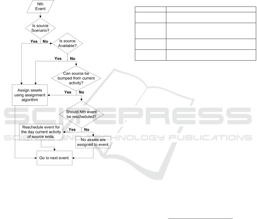
Once a list of events for the iteration has been

built, Tyche will assign assets to each event in a

chronological order. The flow chart in Figure 1

illustrates how Tyche processes each Nth event in

the event list.

Figure 1: Event logic flow chart.

2.2.2 Asset Scoring Criteria

The method by which assets are selected for

assignment is based on an additive cost function.

While this is a myopic policy for meeting a single

requirement by selecting from a list of assets based

on information that is known now and actionable

now (MP:R-AL/KNAN) (Wu et al., 2009), it

provides a great deal of flexibility to mimic the

decisions made by a military scheduler. Additional

model development is planned to include

optimization of asset assignment over the entire

requirements list (events) at a given point in time

and implementing a rolling time-horizon policy for

forecasted demand.

The cost function is calculated for a set of assets

using four scoring criteria that are described in Table

1; each criterion is defined separately for every

scenario phase (for events with an asset source,

levels use a predefined subset of these criteria). The

first set of assets computed that has the highest score

based on the scoring criteria is assigned to the

mission. In the case of a tied score, the first

computed with the score is selected – hence, entry

order is important.

Table 1: Scoring criteria composition.

Criteria Description

Capability

(mandatory)

Number of capability demands that are met at

the required or marginal level.

Capability

Excess

(optional)

Sum of the quality of the capabilities

supplied by the assigned assets that exceed

the capability demand of the scenario phase.

Timeliness

(optional)

Sum of the time delay for all capabilities

provided after the desired response time.

Conflict

(optional)

Sum of the penalties for every asset bumped

to go to the scenario phase.

The cost function for a single asset is simply the

weighted sum of the scores obtained for all selected

scoring criteria. Weights for each criterion are

subjectively established by the user and can be

tailored to try to reproduce the asset selections made

by a military scheduler. A tool is included in the

software to allow the user to preview the ideal asset

selections (assuming unlimited assets and no

timeliness or scheduling conflict) to tune the weights

before a simulation is run. Consider a scenario (s)

with a set of capability demands {D}. An asset with

a set of capability supply {S} will have the cost (C)

components defined in Eqs. (2)-(5), with the

subsequent scaling factors (Sc). The scaling factors

are also weights that are subjectively established by

the user, different from the cost component weights

used in the overall cost function.

⎟

⎠

⎞

⎜

⎝

⎛

∑∑

)()(

5.0

DCC

WWScC

(2)

∑

∉

−=

}{

(S)

ECEC

QScC

(3)

(

)( )

[

]

⎟

⎠

⎞

⎜

⎝

⎛

−Θ−

−=

∑

∈

∉

}{

)(*)(

TSTTST

ScC

(4)

∑

≠

−=

LALA

CDSCSC

,LLScC

)(:

)Penalty( Bump

(5)

The capability score (Eq. 2) is obtained by

summing over the capability demands that are met at

the required level (D(R)) and over those met only at

the marginal level (D(M)). The arbitrary factor 0.5

multiplying the second sum indicates that the

capability met at the required level provides a higher

contribution to the capability score than those only

A STRATEGIC SIMULATION TOOL FOR CAPABILITY-BASED JOINT FORCE STRUCTURE ANALYSIS

met at the marginal level. Furthermore, since the

capability score is obtained from the sum of the

capability weights (W(D), indicating the importance

of the capability to the success of the scenario

phase), capabilities with higher weights will

contribute more to the score.

The excess capability score in Eq. (3) is obtained

by summing over all the capability supplies (S) that

are not requested by the capability demand (

∉

D).

This excess score prevents Tyche from sending too

much capability (too many assets or too capable

assets) to the scenario phase. Excess quality of a

capability that is required by a scenario and provided

by an asset is not taken into account (i.e., if two

assets supply the same capability at different

qualities, both greater than the required quality level,

there is no penalty for selection of the one asset that

exceeds the required level more than the other).

Eq. (4) defines the timeliness score, where T

the desired response time and Θ(T(S)-T

) is the

Heaviside step function. The timeliness score is

obtained by computing the overall delay (T(S)-T

)

required to get all of the capability supplies (S) that

are requested by the capability demand (

∈

D) into

theatre. The summation is normalized by the number

of supplied capabilities.

Finally, the conflict score is obtained by

summing the penalties of all bumped assets in Eq.

(5). The penalty given for bumping the asset is

specified by the user in the asset type definition for

bumping the asset from its current level (L

) to the

desired level (L

). The sum is over all selected assets

(A) for which the current level (L

(A)) is not the

default level. This conflict score favours the

selection of available assets rather than bumping

non-available ones.

The cost function for a group of assets is then the

additive score for each individual asset; it is also a

function of the order in which the assets are

assigned. This will be discussed further in Section

2.2.3.

In addition, a threshold is also established for

each scoring criteria. The threshold is used to reject

poor groups of assets. In other words, if the best

group of assets has an unacceptably low score

component, it is possible to reject it and not send any

assets at all. The threshold allows the user, for

example, to prevent assets from being sent to a six-

month mission to arrive only two days before the

end of the mission. The effect of the thresholds

(Thr) can be summarized as follows. If, for a given

mission, the set of assets with the highest cost

function is a set of k assets, σ(A

,…,A

), then the set

of assets assigned to the mission, σ*, is given in Eq.

(6).

()

⎪

⎩

⎪

⎨

⎧

<∃

otherwise ,...,

*)( | Criterion if 0

1 k

ThrScSign

(6)

Where “0” is the empty set of assets and “Sign”

is a function that returns -1, 0, or 1 based on the

value of the argument (<0,=0,>0).

2.2.3 Asset Assignment Algorithm

The assignment problem consists of matching the

capability demand with the capability supply in an

optimal way, with the objective of maximizing the

cost function. This problem is thus equivalent to

finding an optimal matching on a bipartite weighted

graph. This equivalence follows from the following

definitions (Diestel, 2005):

 A graph is a set of nodes and a set of edges

between nodes. For the assignment problem,

the nodes are given by the set of capability

supplies and capability demands while the

edges are determined from the search domain;

 A weighted graph has a scalar value associated

with every edge. For the assignment problem,

the weight associated with the edge is

computed using the capability and timeliness

scoring criteria as described in Eqs. (2) and

(4);

 A bipartite graph is a graph for which the set of

nodes can be divided into two subsets such

that there is no edge between nodes pertaining

to the same group. For the assignment

problem, the nodes can be divided into the set

of capability demand and the set of capability

supply. Since every edge is between a

capability and a capability demand, the graph

is bipartite;

 A matching on a graph is obtained by selecting

a subset of edges such that no selected edge

has a common node. The assignment of assets

is done by matching each capability demand

with one, and only one, capability supply. It

thus corresponds to selecting a matching on

the graph. Every asset for which at least one

capability supply is adjacent to an edge

pertaining to the matching belongs to the set

of selected assets.

Only the capability score and timeliness score

can be assigned as a weight associated with the

edges. This is possible because these two scores are

given as a sum over the capability demands that are

ICORES 2012 - 1st International Conference on Operations Research and Enterprise Systems

matched. The excess and conflict score cannot be

obtained through a distributed sum along the edges

pertaining to the matching. Thus, if the excess and

conflict score do not belong to the selected scoring

criteria then the optimal matching corresponds

directly to the highest weight matching, which is a

well-known problem in graph theory (Diestel, 2005).

In particular, the backtracking and backjumping

algorithm has been applied successfully to this type

of problem (Wolf, 2006). Because the weights for

the excess and conflict scoring criteria are typically

small, this algorithm should produce solutions that,

while not optimal, are “good enough”.

Because there are typically few asset types that

can satisfy a given set of capabilities, the user can

exploit this information to define a restricted search

domain. An enumerated search is then performed to

determine which assets to assign. Tailoring of the

search domain adds a significant amount of

flexibility for assignment selection, increasing the

capability of the program. The enumerated search is

guaranteed to select the best available asset when

only one asset is required for a scenario. If more

than one asset is required, it is possible that the

highest ranked combination of available assets is not

assigned, because the search is conducted on an

asset-by-asset basis. The next asset that adds the

most to the total score, based on the remaining

capability demand, is assigned.

The selection of assets is also done in a multi-

layered way. At each layer, assets are selected to

meet the capability demands that were introduced at

the previous layer. If, at some layer, the capability

demands cannot be met, then the algorithm

backtracks to the previous layer and selects a

different group of assets. At each layer, after a group

of assets has been selected, the algorithm checks for

redundancy. If redundant assets are found, then the

redundant asset is removed and replaced by the new

asset that can provide the capability that the

redundant asset was providing and the algorithm

backjumps to the layer where the redundant asset

was selected.

2.3 Output and MOP

The results of the Monte Carlo simulation are output

so that operational schedules from individual

iterations can be viewed in text or graphical format.

This allows for detailed examination of asset

assignment, scheduling conflicts, and mission

timing. Upon completion of the simulation run,

statistics are generated for asset usage, scenario

assignments, and capability fulfillment. A

capability-based risk measure is introduced to

aggregate the results into a single MOP for force

structure comparisons.

2.3.1 Statistical Information

Asset statistics collect information on the

assignment of individual force structure assets in

terms of average duration and standard deviation of

the duration spent at a given level. While the user

must reconstruct which levels correspond to which

scenario phases, the data output is generalized for

use across all military services.

Scenario statistics indicate the average frequency

of occurrence of scenario phases and the percentage

of time that particular combinations of assets (or no

assets) are being sent.

Capability statistics are the primary indicator of

the ability of a force structure to meet scenario

demand. For each scenario phase, the percentage of

time that capabilities are not met at the required and

marginal levels are reported.

2.3.2 Capability-based Risk Assessment

Maintaining the focus on capability-based planning,

an assessment of the risk associated with a particular

force structure can be derived using the probability

that capabilities are not met, and frequency of

scenario occurrence. The risk is defined in Eq. (7),

where the mean yearly political risk (R) for a given

scenario (s) is defined as the product of the annual

frequency of occurrence (f), the impact (I) of failure

to provide capability, and the probability the

capability supply deployed is inadequate (P). The

risk is then summed over all scenarios.

∑

sss

PIf R

(7)

The first factor is assessed by averaging the

number of times the scenario occurs yearly across all

iterations. The second factor, known as impact

score, can be provided as a subjective input by

SME’s. This allows the risk assessment to

incorporate military judgement, often critical to

balance the perceived effect of low impact-high

frequency and high impact-low frequency scenarios.

The third and final factor (P

) is calculated from Eq.

(8). The probability that the capability supply is

inadequate can be defined in several ways,

depending on how risk-averse the assessment should

be. In general, it is a weighted summation of the

percentage of time (P

Tyche

) that the scheduler fails to

provide capability to a scenario with a given asset

assignment (A).

A STRATEGIC SIMULATION TOOL FOR CAPABILITY-BASED JOINT FORCE STRUCTURE ANALYSIS

∑

TycheAs

APwP )(*

(8)

Given that the Tyche scheduler can assign assets

to meet capability at different levels, one highly risk-

averse method would be to utilize three categories:

where, due to force structure limitations, Tyche fails

to assign assets altogether (A=0), and where at least

one capability demand is not met at the required

(A=R’) and marginal level (A=M’). The weights for

each of the categories of capability failure can also

be provided by SME input. In the case study, it will

be assumed that w

= 1.0, w

R’

= 0.5 and w

M’

= 0.1.

The statistical nature of the risk measure also

implies that there is an error on the estimation of the

average. It is reported as twice the standard

deviation (σ) of the mean distribution, where σ is

estimated by the square root of the sample variance

of the risk distribution divided by the number of

iterations.

3 A CASE STUDY

Utilizing a simple case study, it is possible to

illustrate the kinds of results Tyche can produce, as

well as the types of problems that can be analysed.

The case study is built around hypothetical asset

types and scenarios, and the capabilities attributed to

these assets are not intended to model capabilities of

real force assets.

In this example, five generic capabilities (A, B,

C, D, E) were created, along with two crewing and

one transport capabilities for modelling

dependencies. Five asset types (Air Asset, Air Crew,

Sea Asset, Sea Crew, and Special Operations Force)

can supply these capabilities, at various levels

shown in Table 2. The Air Asset requires an Air

Crew with a quantity of 3 persons, and can provide

transport for up to 10 persons. The Sea Asset

requires a Sea Crew, with a quantity of 70, and can

provide transport for 100 persons. The Special

Operations Force (SOF) is composed of 6 persons,

and can be transported on either Air or Sea Assets.

Table 2: Asset capability supply.

Asset Type Capability Quality Quantity

Air Asset A

0.8

0.7

0.2

Sea Asset A

0.7

0.6

0.9

SOF E 1.0 1

Air Assets were modelled to have a 50% chance

of requiring maintenance after use in a scenario,

with a duration determined from a triangular

distribution with minimum, most likely and

maximum values of 1, 2, and 10 days. They were

also restricted for use in 100 of every 365 days. The

Sea Asset has a Short Work Period of 18-20-25 days

5 times per year. It also has a Docking Work Period

of 100-180-365 days once every 5 years. Both Air

and Sea Crews were constrained to take a quality-of-

life break after every scenario for 5-5-10 days.

There were two bases: Air 1 and Sea 1,

collocated together. There were four possible

theatres, some favouring the assignment of air assets

and others that are unbiased. Three scenarios (S1-

S3) were defined to occur at two or more possible

theatres, with requirements from Table 3. The

scenario search domain was the same for all,

including Air Assets from Air 1, Sea Assets from

Sea 1, and SOF from Air 1.

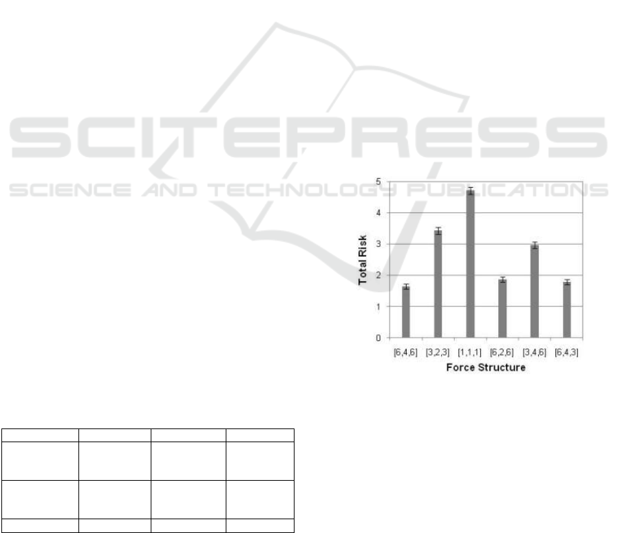
Six force structures were tested. It was assumed

that there was one crew per platform, and force

structures are labelled according to the number of

[Air Assets, Sea Assets, SOF]. The first three

structures, [6,4,6], [3,2,3] and [1,1,1] looked at

decreasing fleet sizes across all assets. Three

additional structures reduced a single asset type from

the largest, [6,2,6], [3,4,6], and [6,4,3]. The risk

measure was computed using three for impact score,

with values of 1.0 for S1, 1.5 for S2, and 5.0 for S3,

and is shown in Figure 2.

Figure 2: Case study results.

As illustrated, the risk of not being able to fulfil

scenario capability requirements increases with

decreasing fleet size. The simple parametric

decrease in assets of a given type indicates that force

structure [6,2,6] and [6,4,3] do not have a

statistically significant difference in performance,

and are near the large [6,4,6] structure. However,

when Air Assets are removed [3,4,6], the risk

increases sharply.

This case study is representative of the force

ICORES 2012 - 1st International Conference on Operations Research and Enterprise Systems

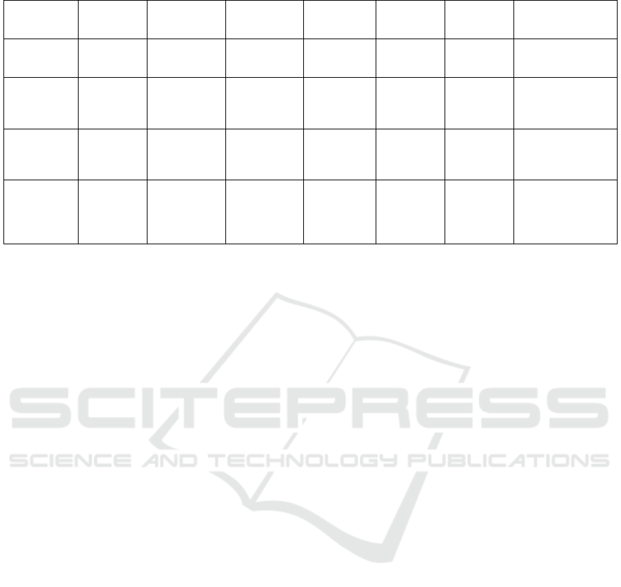
Table 3: Scenario timing and capability demand.

Scenario:

Phase

Type,

Frequency

Theatre,

Probability

Duration,

Response

Time (Days)

Capability,

Quantity

Required,

Marginal

Quality

Weight (All

Non-

Essential)

Scoring Criteria,

Weight, Scale,

Threshold

S1:P1 Random

3.0 / year

1, 0.2

2, 0.8

20-30-60

A, 1

B, 15

C, 2

0.8, 0.4

0.7, 0.2

0.4, 0.1

Capability,10,1,1

Conflict,1,1,100

S2:P1 Scheduled

1.0 / year

Starting on

Day 30

1, 0.25

2, 0.25

3, 0.25

4, 0.25

30-60-90

A, 1

C, 2

E, 2

0.6, 0.4

0.4, 0.1

1.0, 1.0

Capability,10,1,1

Conflict,1,1,100

Timeliness,1,1,20

S3:P1 Random

0.33 / year

3, 0.8

4, 0.2

90-150-180

A, 1

B, 15

C, 2

E, 4

0.9, 0.4

0.7, 0.2

0.4, 0.1

1.0, 1.0

Capability,10,1,1

Conflict,1,1,100

Timeliness,5,1,8

S3:P2 Follow-on,

With P1

duration ≥

150 days

Same as P1 90-150-180

No overlap

with P1

A, 1

B, 15

C, 2

D, 1

E, 4

0.9, 0.4

0.7, 0.2

0.4, 0.1

0.5, 0.3

1.0, 1.0

Capability,10,1,1

Conflict,1,1,100

Timeliness,5,1,8

structure analysis that can be performed with Tyche,

as well as options analysis around force structures of

interest. While Tyche is not integrated into an

optimization framework, simulation optimization to

determine the optimal fleet with respect to some

objective (minimum risk, structure size, cost, etc.)

can still be performed, albeit in a less efficient way.

Tyche is also useful for performing options

analysis, capability gap analysis, testing new

capability architectures, and evaluating force

structure performance in the face of changing

requirements. As well, the rate of usage of assets can

be examined to determine the effects of readiness

and sustainment policies on performance in

operations. For example, in the case study, the Sea

Asset goes through a number of work periods. The

length and frequency can be varied to determine the

effect on risk. Similarly, with crews, operations and

personnel tempo constraint policies can be varied.

4 CONCLUSIONS

This paper described a Monte Carlo discrete event

simulation for joint force structure analysis. The

Tyche tool is currently used by DRDC CORA and,

while it has not yet been employed for a formal joint

force structure study, it exhibits potential advantages

for strategic level capability-based planning.

Development is already underway to rectify known

modelling limitations. Additional research avenues

include optimization of asset assignment over the

entire requirements list at a given point in time and

implementing a rolling time-horizon policy for

forecasted demand.

ACKNOWLEDGEMENTS

The authors would like to thank Alex Bourque,

Pawel Michalowski, Carolyn Augusta, Dave

Heppenstall, Alain Forget, Debbie Blakeney, Evan

DeCorte, R.M.H. Burton, and Geordie MacDonald

for their roles in the development of Tyche.

REFERENCES

Abbass, H., Bender, A., Baker, S. , Sarker, R. A. Year.

Anticipating future scenarios for the design of

modularised vehicle and trailer fleets. In: SimTecT,

2007 Brisbane, Australia.

Baker, S. F., Morton, D. P., Rosenthal, R. E. , Williams, L.

M. 2002. Optimizing Military Airlift. Operations

Research, 50, 582-602.

Brown, G. G., Clemence, R. D., Teufert, W. R. , Wood, R.

K. 1991. An optimization model for modernizing the

army’s helicopter fleet. INTERFACES, 21, 39-52.

Bulut, G. 2001. Robust Multi-Scenario Optimization of an

Air Expeditionary Force Force Structure Applying

Scatter Search to the Combat Forces Assessment

Model. Air Force Institute of Technology.

Cortez, L. A. , Kaiser, T. J. 1991. U.S. Coast Guard Fleet

Mix Planning: A Decision Support System Prototype.

Master of Science in Information Systems, Naval

Postgraduate School.

Crary, M., Nozick, L. K. , Whitaker, L. R. 2002. Sizing

the US destroyer fleet. European Journal of

Operational Research, 136, 680-695.

Davis, P. K. 2002. Analytic architecture for capabilities-

based planning, mission-system analysis, and

transformation. Santa Monica, CA: RAND

Corporation.

A STRATEGIC SIMULATION TOOL FOR CAPABILITY-BASED JOINT FORCE STRUCTURE ANALYSIS

Diestel, R. 2005. Graph Theory. Graduate Texts in

Mathematics, Vol. 173. 3rd ed. Heidelberg: Springer-

Verlag.

Dugan, K. 2007. Navy Mission Planner. Master of Science

in Operations Research, Naval Postgraduate School.

Farr, J. V., Nelson, M. S. , Diaz, A. A. 1994. Resource

Allocation Methodology to Support Mission Area

Analysis. West Point, NY: United States Military

Academy.

Fildes, L. 2006. A Decision Support Tool for the

Procurement and Planning of Royal Naval Ships.

Master of Science in Operational Research, University

of Southampton.

Gallagher, M. A. , Kelly, E. J. 1991. A New Methodology

for Military Force Structure Analysis. Operations

Research, 39, 877-885.

Gauthier, Y., Wardrop, W., Price, A. , Lawrence, A. 2008.

The size of MARS: quantifying requirements for the

Royal Navy’s future afloat support fleet. 25th

International Symposium on Military Operational

Research. Cranfield University.

Greer, W. L., Kaufman, A. I., Levine, D. B., Nakada, D.

Y. , Nance, J. F. 2005. Exploration of Potential Future

Fleet Architectures. Alexandria, VA: Institute for

Defense Analyses.

Horn, M. E. T., Jiang, H. , Kilby, P. 2007. Scheduling

patrol boats and crews for the Royal Australian Navy.

Journal of the Operational Research Society, 58,

1284-1293.

Klerman, J. A., Ordowich, C., Bullock, A. M. , Hickey, S.

2008. The RAND SLAM program. RAND National

Defense Research Institute.

Mattila, V., Virtanen, K. , Raivio, T. 2008. Improving

Maintenance Decision Making in the Finnish Air

Force Through Simulation. INTERFACES, 38, 187-

201.

Mattock, M., Schank, J., Stucker, J. , Rothenberg, J. 1995.

New capabilities for strategic mobility analysis using

mathematical programming, RAND Corporation.

Salmeron, J., Wood, R. K. , Morton, D. P. 2009. A

Stochastic Program For Optimizing Military Sealift

Subject To Attack. Military Operations Research, 14,

19-39.

Taylor, B. , Lane, A. 2004. Development of a Novel

Family of Military Campaign Simulation Models. The

Journal of the Operational Research Society, 55, 333-

339.

Walmsley, N. S. , Hearn, P. 2004. Balance of Investment

in Armoured Combat Support Vehicles: An

Application of Mixed Integer Programming. The

Journal of the Operational Research Society, 55, 403-

412.

Wesolkowski, S. , Billyard, A. 2008. The Stochastic Fleet

Estimation (SaFE) model. Proceedings of the 2008

Spring simulation multiconference.

Ottawa, Canada:

Society for Computer Simulation International.

Whitacre, J. M., Bender, A., Baker, S., Fan, Q., Sarker, R.

A. , Abbass, H. Year. Network Topology and Time

Criticality Effects in the Modularised Fleet Mix

Problem. In: SimTecT, 2008 Melbourne, Australia.

Wolf, A. 2006. Intelligent Search Strategies Based on

Adaptive Constraint Handling Rules. Theory and

Practice of Logic Programming, 6, 213-224.

Wu, T. T., Powell, W. B. , Whisman, A. 2009. The

optimizing-simulator: An illustration using the

military airlift problem. ACM Transactions on

Modeling and Computer Simulation, 19, 1-31.

Zadeh, H. S. 2009. NaMOS; Scheduling Patrol Boats and

Crews for the Royal Australian Navy. 2009 IEEE

Aerospace Conference. Big Sky, MT.

ICORES 2012 - 1st International Conference on Operations Research and Enterprise Systems