
SCALABLE CORPUS ANNOTATION BY GRAPH CONSTRUCTION
AND LABEL PROPAGATION
Thomas Lansdall-Welfare, Ilias Flaounas and Nello Cristianini
Intelligent Systems Laboratory, University of Bristol, Woodland Road, Bristol, U.K.
Keywords:
Text categorisation, Graph construction, Label propagation, Large scale.
Abstract:
The efficient annotation of documents in vast corpora calls for scalable methods of text classification. Rep-
resenting the documents in the form of graph vertices, rather than in the form of vectors in a bag of words
space, allows for the necessary information to be pre-computed and stored. It also fundamentally changes
the problem definition, from a content-based to a relation-based classification problem. Efficiently creating
a graph where nearby documents are likely to have the same annotation is the central task of this paper. We
compare the effectiveness of various approaches to graph construction by building graphs of 800,000 vertices
based on the Reuters corpus, showing that relation-based classification is competitive with Support Vector Ma-
chines, which can be considered as state of the art. We further show that the combination of our relation-based
approach and Support Vector Machines leads to an improvement over the methods individually.
1 INTRODUCTION
Efficiently annotating new documents coming from a
data stream is an important problem in modern data
management. Real world text mining and analysis
systems, such as news monitoring systems like ‘News
Outlets Analysis and Monitoring system’ (NOAM)
(Flaounas et al., 2011), Lydia (Lloyd et al., 2005)
and the ‘Europe Media Monitor’ (EMM) (Steinberger
et al., 2009) would benefit from an approach that can
handle annotation on a large scale while being able
to adapt to changes in the data streams. A classical
approach is to develop content-based classifiers, e.g.
Support Vector Machines (SVMs), specialised in the
detection of specific topics (Joachims, 1998). One of
the key problems in this approach is that the classifi-
cations are not affected by subsequent documents, un-
less the classifiers are retrained, and that entirely new
topics cannot be introduced unless a new classifier is
developed. We are interested in the situation where
the annotation of a corpus improves with time, that
is with receiving new labelled data. We want the ac-
curacy of existing labels to improve with more data,
where old errors in classification are possibly being
amended, and if entirely new topic labels start being
used in a data stream, the system will be able to ac-
commodate them automatically. The deployment of
such methods for real world textual streams, such as
news feeds coming from the Web where the feed is
constantly updated, requires an ability to track them
in real time, independent of the size of the corpus.
The na¨ıve approach to graph construction, comparing
all documents to all documents or building a complete
kernel matrix (Shawe-Taylor and Cristianini, 2004),
will not work in large scale systems due to high com-
putational complexity. The cost of label propagation
is also an important factor on the time needed to pro-
cess the incoming documents.
In this paper we focus on textual data and present
a method to propagate labels across documents by
creating a sparse graph representation of the data,
and then propagating labels along the edges of the
graph. There is a tendency for research to focus on the
method of propagating the labels, taking for granted
that the graph topology is given in advance (Herbster
et al., 2009; Cesa-Bianchi et al., 2010b). In reality,
unless working with webpages, textual corpora rarely
have a predefined graph structure. Graph construc-
tion alone has a worst case cost of O (N
2
) when using
a na¨ıve method due to the calculation of the full N×N
pairwise similarity matrix. Our proposed method can
be performed efficiently by using an inverted index,
and in this way the overall cost of the method has a
time complexity of O (N logN) in the number of doc-
uments N.
We test our approach by creating a graph of
800,000 vertices using the Reuters RCV1 corpus
(Lewiset al., 2004), and we compare the quality of the
25
Lansdall-Welfare T., Flaounas I. and Cristianini N. (2012).
SCALABLE CORPUS ANNOTATION BY GRAPH CONSTRUCTION AND LABEL PROPAGATION.
In Proceedings of the 1st International Conference on Pattern Recognition Applications and Methods, pages 25-34
DOI: 10.5220/0003728700250034
Copyright
c
SciTePress

label annotations obtained by majority voting against
those obtained by using SVMs. We chose to com-
pare the graph-based methods to SVMs because they
are considered the state of the art for text categorisa-
tion (Sebastiani, 2002). We show that our approach
is competitive with SVMs, and that the combination
of our relation-based approach with SVMs leads to an
improvement in performance over either of the meth-
ods individually. Further to this, we show that the
combination of the approaches does not lead to a de-
crease in performance, relative to the weakest of the
approaches, i.e. the combination always gives an im-
provementover at least one of the methods on its own.
It is also important to notice that our methods can be
easily distributed to multiple machines.
This paper is organised as follows: Section 2 out-
lines graph construction, detailing methods of us-
ing an inverted index for graph construction, along
with various methods for maintaining sparsity of the
graph. Section 3 outlines the Label Propagation (LP)
method and Online Majority Voting (OMV), a natu-
ral adaption of LP for an online setting. Section 4
describes the implementation details concerning the
inverted index and edge lists, while Sect. 5 covers
our experimental comparison of our presented meth-
ods with Support Vector Machines on the Reuters cor-
pus before showing an improvement by combining
the methods. Finally, in Sect. 6 we discuss the ad-
vantages of a graph-based approach and summarise
our findings before posing some directions for future
work in the area.
1.1 Related Work
There is a growing interest in the problem of prop-
agating labels in graph structures. Previous work
by Angelova and Weikum (Angelova and Weikum,
2006) extensively studied the propagation of labels
in web graphs including a metric distance between
labels, and assigning weights to web links based
upon content similarity in the webpage documents.
Many alternative label propagation algorithms have
also been proposed over the years, with the survey
(Zhu, 2007) giving an overview of several different
approaches cast in a regularisation framework. A
common drawback of these approaches is the pro-
hibitively high cost associated with label propaga-
tion. A number of recent works on label propaga-
tion (Herbster et al., 2009; Cesa-Bianchi et al., 2010a;
Cesa-Bianchi et al., 2010b) concentrate on extracting
a tree from the graph, using a very small number of
the neighbours for each node.
While many graph-based methods do not address
the problem of the initial graph construction, assum-
ing a fully connected graph is given, or simply choos-
ing to work on data that inherently has a graph struc-
ture, there is a large number of papers dedicated to
calculating the nearest neighbours of a data point.
One such approximate method, NN-Descent (Dong
et al., 2011), shows promising results in terms of ac-
curacy and speed for constructing k-Nearest Neigh-
bour graphs, based upon the principle that ‘a neigh-
bour of a neighbour is also likely to be a neighbour’.
The All-Pairs algorithm (Bayardo et al., 2007) tack-
les the problem of computing the pairwise similar-
ity matrix often used as the input graph structure in
an efficient and exact manner, showing speed im-
provementsover another inverted-list based approach,
ProbeOpt-sort (Sarawagi and Kirpal, 2004) and well-
known signature based methods such as Locality Sen-
sitive Hashing (LSH) (Gionis et al., 1999).
In this paper we take a broader overview, consid-
ering both the task of creating a graph from text docu-
ments, and then propagating labels for text categorisa-
tion simultaneously. We are interested in an approach
that can be applied to textual streams, with the previ-
ously mentioned additional benefits offered by mov-
ing away from classical content-based classifiers.
2 GRAPH CONSTRUCTION
Graph construction X → G deals with taking a corpus
X = {x
1
, . . . , x
n
}, and creating a graph G = (V, E,W),
where V is the set of vertices with document x
i
being
represented by the vertex v
i
, E is the set of edges, and
W is the edge weight matrix. There are several ways
the construction can be adapted, namely the choice of
distance metric and the method for maintaining spar-
sity.
The distance metric is used to determine the edge
weight matrix W. The weight of an edge w
ij
encodes
the similarity between the two vertices v
i
and v
j
. The
choice of metric used is mostly task-dependent, re-
lying on an appropriate selection being made based
upon the type of data in X . A common measure used
in text, such as cosine similarity (Tan et al., 2006),
may not be appropriate for other data types, such as
when dealing with histogram data where the χ
2
dis-
tance is more meaningful (Zhang et al., 2007).
Typically, a method for maintaining sparsity is re-
quired since it is not desirable to work with fully
connected graphs for reasons of efficiency, and sus-
ceptibility to noise in the data (Jebara et al., 2009).
This can be solved by working with sparse graphs,
which are easier to process. Two popular methods
for achieving sparsity include k-nearest neighbour
(kNN) and ε-neighbourhood, both utilizing the local
ICPRAM 2012 - International Conference on Pattern Recognition Applications and Methods
26
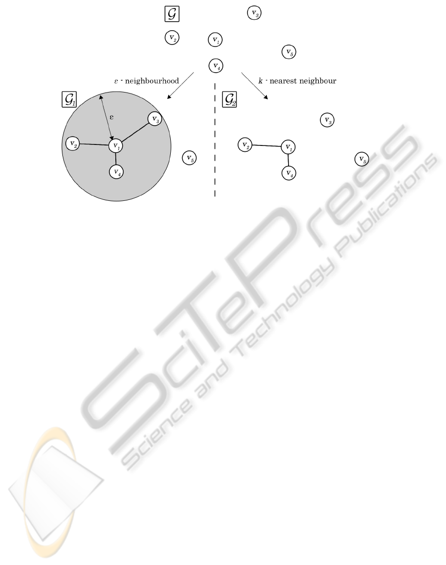
Figure 1: Illustration of an example where two graphs, G
1
and G
2
, are being constructed from graph G using the two
methods we investigate: ε-neighbourhood and k-nearest neighbour. In the example, the possible edges for vertex v
i
are being
considered. The ε-neighbourhood method adds all edges which connect v
1
to a vertex inside the grey circle which visualises
the radius ε. The k-nearest neighbour method ranks the closeness of the adjacent vertices with respect to a given similarity
measure, then adds edges to the closest k vertices. For this example, k = 2.
neighbourhood properties of each vertex in the graph
(Carreira-Perpinan and Zemel, 2004; Jebara et al.,
2009; Maier et al., 2009). Local neighbourhoodmeth-
ods are important for efficiencysince a data point only
relies on information about other points close by, with
respect to the distance metric, to determine the neigh-
bours of a vertex. This means that no global proper-
ties of the graph need to be calculated over the entire
graph each time a new vertex is added, a considera-
tion that has implications both for the scalability and,
more generally, for parallelisation.
The first step of creating the graph usually in-
volves calculating the pairwise similarity score be-
tween all pairs of vertices in the graph using the ap-
propriately chosen distance metric. Many studies as-
sume that it is feasible to create a full N × N dis-
tance matrix (Jebara et al., 2009) or that a graph is al-
ready given (Herbster et al., 2009; Cesa-Bianchi et al.,
2010b). This assumption can severely limit the size
of data that is managable, limited by the O (N
2
) time
complexity for pairwise calculation. Construction of
a full graph Laplacian kernel, as required by standard
graph labelling methods (Belkin et al., 2004; Herbster
and Pontil, 2007; Zhu et al., 2003) is already compu-
tationally challenging for graphs with 10,000 vertices
(Herbster et al., 2009). Jebara et al. (Jebara et al.,
2009) introduce β-matching, an interesting method of
graph sparsification where each vertex has a fixed de-
gree β and show an improved performance over k-
nearest neighbour, but at a cost to the complexity of
the solution and the assumption that a fully connected
graph is given.
We can overcome the issue of O (N
2
) time com-
plexity for computing the similarity matrix by using
an alternative method, converting the corpus into an
inverted index where each term has a pointer to the
documents the term appears within. The advantage
of this approach is that the corpus is mapped into a
space based upon the number of terms, rather than
number of documents. This assumption relies on the
size of the vocabulary |t| being much smaller than the
size of the corpus. According to Heaps’ Law (Heaps,
1978), the number of terms |t| appearing in a corpus
grows as O (N
β
), where β is a constant between 0 and
1 dependent on the text. Some experiments (Araujo
et al., 1997; Baeza-Yates and Navarro, 2000) on En-
glish text show that β is between 0.4 and 0.6 in prac-
tice. The inverted index can be built in O (NL
d
) time
where L
d
is the average number of terms in a docu-
ment, with a space complexity of O (NL
v
) where L
v
is the average number of unique terms per document
(Yang et al., 2003).
Finding the neighbours of a document is also triv-
ial because of the inverted index structure. A classical
approach is to use the Term Frequency-Inverse Doc-
ument Frequency (TF-IDF) weighting (Salton, 1989)
to calculate the cosine similarity between two docu-
ments. This can be performed in O (L
d
log|t|) time for
each document by performing L
d
binary searches over
the inverted index. Assuming β from Heaps’ Law is
the average value of 0.5, the time complexity for find-
ing the neighbours of a document can be rewritten as
SCALABLE CORPUS ANNOTATION BY GRAPH CONSTRUCTION AND LABEL PROPAGATION
27

O (
L
d
2
logN). Therefore, there is a total time complex-
ity O (N +
NL
d
2
logN) for building the index and find-
ing the neighbours of all vertices in the graph. This
is equivalent to O (N logN) under the assumption that
the average document length L
d
is constant.
A further advantage of this method is that the
number of edges per vertex is limited a priori, since
it is infeasible to return the similarity with all docu-
ments in the inverted index for every document. This
allows the construction of graphs that are already
sparse, rather than performing graph sparsification to
obtain a sparse graph from the fully connected graph,
e.g. (Jebara et al., 2009).
We investigate two popular local neighbour-
hood methods, k-nearest neighbour (kNN) and ε-
neighbourhood, for keeping the graph sparse during
the initial construction phase and also when new ver-
tices are added to the graph (Carreira-Perpinan and
Zemel, 2004; Jebara et al., 2009; Maier et al., 2009).
Figure 1 shows intuitively how each of the methods
chooses the edges to add for a given vertex. The first
method, kNN, connects each vertex to the k most sim-
ilar vertices in V, excluding itself. That is, for two
vertices v
i
and v
j
, an edge is added if and only if the
similarity between v
i
and v
j
is within the largest k re-
sults for vertex v
i
. The second method we investigate,
ε-neighbourhood, connects all vertices within a dis-
tance ε of each other, a similar approach to classical
Parzen windows in machine learning (Parzen, 1962).
This places a lower bound on the similarity between
any two neighbouring vertices, i.e. only edges with a
weight abovethe threshold ε are added to the graph. A
simple way of visualising this is by drawing a sphere
around each vertex with radius ε, where any vertex
falling within the sphere is a neighbour of the vertex.
While the first method fixes the degree distribution of
the network, the second does not, resulting in funda-
mentally different topologies. We will investigate the
effect of these topologies on labelling accuracy.
3 LABEL PROPAGATION
Label propagation aims to use a graph G = (V, E,W)
to propagate topic labels from labelled vertices to un-
labelled vertices. Each vertex v
i
can have multiple
topic labels, i.e. a document can belong to more
than one category, and each label is considered in-
dependently of the other labels assigned to a ver-
tex. The labels assigned to the set of labelled ver-
tices Y
l
= {y
1
, . . . , y
l
} are used to estimate the labels
Y
u
= {y
l+1
, . . . , y
l+u
} on the unlabelled set.
Carreira-Perpinan et al. (Carreira-Perpinan and
Zemel, 2004) suggest constructing graphs from en-
sembles of minimum spanning trees (MST) as part
of their label propagation algorithm, with their two
methods Perturbed MSTs (PMSTs) and Disjoint
MSTs (DMSTs), having a complexity of approxi-
mately O (TN
2
logN) and O (N
2
(logN + t)) respec-
tively, where N is the number of vertices, T is the
number of MSTs ensembled in PMSTs, and t is the
number of MSTs used in DMSTs, typically t <<
N
2
.
However, to the best of the authors’ knowledge, no
studies have performed experiments on constructed
graphs with more than several thousand vertices, with
the exception of Herbster et al. (Herbster et al., 2009)
who build a shortest path tree (SPT) and MST for a
graph with 400,000 vertices from Web pages. Herb-
ster et al. (Herbster et al., 2009) also note that con-
structing their MST and SPT trees using Prim and Di-
jkstra algorithms (Cormen et al., 1990) respectively
takes O (NlogN+|E|) time, with the general case of a
non-sparse graph having a time complexity of Θ(N
2
).
In this paper we adopt Online Majority Voting
(OMV) (Cesa-Bianchi et al., 2010b), a natural adap-
tation of the Label Propagation (LP) algorithm (Zhu
et al., 2003), as our algorithm for the label propaga-
tion step due to its efficiency and simplicity. OMV is
based closely upon the locality assumption, that ver-
tices that are close to one another, with respect to a
distance or measure, should have similar labels. Each
vertex is sequentially labelled as the unweighted ma-
jority vote on all labels from the neighbouring ver-
tices. The time complexity for OMV is Θ(|E|), a no-
table reduction from the O (kN
2
) required for LP al-
gorithm, where k is the neighbours per vertex. The
complexity being dependent on the number of edges
in the graph further benefits from the a priori limit we
impose upon the maximum edges per vertex, ensuring
that |E| = bN for some maximum edge limit b.
4 IMPLEMENTATION
The data structures for the implementation of the pro-
posed methods can be separated into two individual
parts. Firstly, an inverted index is built that is used for
the efficient calculation of neighbours for a document,
and secondly, an edge list is maintained in a relational
database, allowing for queries to be executed on the
graph topology.
For the experiments in this paper, the inverted in-
dex is implemented using the open source Apache
Lucene
1
software. An inverted index is a data struc-
ture where, as previously described, a list of every
term in the corpus is maintained with a pointer (also
1
Open source implementation of an inverted index.
Available at: http://lucene.apache.org/
ICPRAM 2012 - International Conference on Pattern Recognition Applications and Methods
28
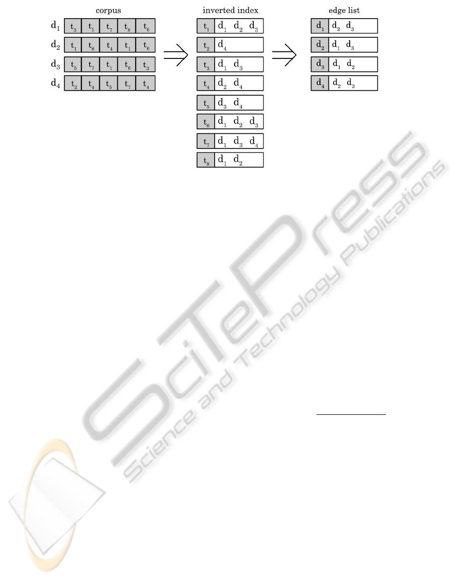
Figure 2: Illustration of the conceptual change in how the data is stored for the inverted index and edge list approach. This
example shows a corpus containing four documents (d
1
, d
2
, d
3
, d
4
) with terms t
1
,t
2
, . . . ,t
8
being converted into an inverted
index with postings to each of the documents originally containing the term. From the inverted index, an edge list can then
be generated linking the documents (d
1
, d
2
, d
3
, d
4
) into a graph. In this example, the edge list depicts a k-Nearest Neighbour
graph where k = 2.
known as a posting) to each document that contains
that term. The inverted index can be stored in main
memory for small corpora, significantly speeding up
the document search procedure, or on disk for larger
corpora.
The edge list generated from the inverted index is
stored in a relational database. For the experiments in
this paper MySQL is used allowing for neighbours of
a vertex to be retrieved quickly by querying the edge
list table for the relevant vertex identifier. Figure 2
illustrates the structure of an inverted index and the
edge list generated from it.
We adapted the source code of Lucene to support
cosine similarity between documents, since it is ini-
tially optimised for document retrieval, rather than
document comparison. The SVMs were deployed us-
ing the LibSVM toolbox (Chang and Lin, 2001).
5 EXPERIMENTS AND
EVALUATION
We present an experimental study of the feasibility of
our approach on a large data set, the Reuters RCV1
corpus (Lewis et al., 2004). We split the corpus into
a training and test set, where the test set is the last
seven weeks of the corpus, and the training set covers
everything else. The test set is further subdivided into
seven test weeks.
For the graph-based methods, the hyperparam-
eters k and ε require careful selection in order to
achieve comparable performance with current meth-
ods. This is the most expensive step as it often
requires a search of the parameter space for the
best value. We use Leave-One-Out Cross Validation
(LOO-CV) on the training set to tune the parame-
ters. This involves constructing graphs for a range
of values of k and ε on the training set by iterating
over all vertices, predicting the labels of the vertex
based upon the majority vote of its neighbours. The
predictions are checked against the true labels, with
the highest performing parameter value being chosen.
The performance was evaluated using the F
1
Score,
which is the harmonic mean of the precision and re-
call, a widely used performance metric for classifi-
cation tasks (Steinbach et al., 2000). Formally, it is
defined as
F
1
= 2·
precision· recall
precision+ recall
. (1)
The precision and recall on the training set were cal-
culated by summing together the contingency matri-
ces for each topic, giving an F
1
Score for each pa-
rameter value across all topics. For the test sets, all
F
1
Scores reported are the individual topic F
1
Scores
averaged over the 50 most common topics. The
best parameters for each method were also recorded
for each topic individually, allowing for a multi-
parameter graph where each label has a different pa-
rameter value. This could be thought of as each la-
bel being able to travel a certain distance along each
edge. It was however found that the multi-parameter
approach only led to a small increase in performance
at additional cost to the complexity of the solution
since multiple graphs need to be constructed.
We trained one SVM per topic using the Cosine
kernel, which is a normalised version of the Lin-
ear kernel (Shawe-Taylor and Cristianini, 2004). For
SCALABLE CORPUS ANNOTATION BY GRAPH CONSTRUCTION AND LABEL PROPAGATION
29
0 0.2 0.4 0.6 0.8 1
0
20
40
60
80
100
ε−Neighbourhood Threshold
F
1
Score
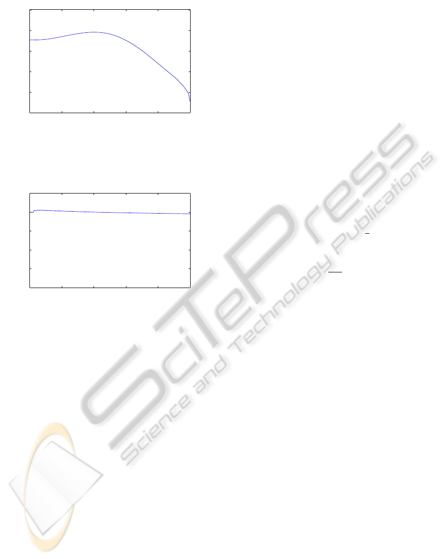
Figure 3: This figure shows the F
1
performance averaged
across the 50 most common topics evaluated on the training
set using LOO-CV for ε = {0, 0.01, . . . , 1.00}. It can been
seen that there is a curve with a peak at ε = 0.4.
0 20 40 60 80 100
0
20
40
60
80
100
k−Nearest Neighbours
F
1
Score
Figure 4: This figure shows the F
1
performance for the
50 most common topics evaluated on the training set us-
ing LOO-CV for k = {1, 2, . . . , 100}. It can been seen that
the line peaks relatively quickly, at k = 5.
each topic, training used a randomly selected 10, 000
positive examples, and a randomly selected 10, 000
negative examples picked from the training set. The
examples were first stemmed and stop words were re-
moved as for the graph-based methods. The last week
of the training corpus was used as a validation set to
empirically tune the regularisation parameter C out of
the set [0.01, 0.05, 0.1, 0.5, 1, 5, 10, 100]. For each
topic, C was tuned by setting it to the value achieving
the highest F
1
performance on that topic in the vali-
dation set. We report the performance on the test set.
5.1 Combining Graph-based and
Content-based Classification
Further to the comparison of the graph-based meth-
ods with SVMs, an ensemble (Dietterich, 2000) of the
graph-based and content-based classification methods
was evaluated. For each vertex, a majority vote for
each class label c is taken by counting the supporting
votes from k votes of the kNN method, supplemented
with s votes from the SVMs for a total of υ = k + s
votes. That is, each vertex has the k votes from the
kNN method, but also s votes assigned by the SVMs.
The number of votes from the SVM is chosen in the
interval s = [0, k + 1]. This moves the combination
method from purely graph-based at s = 0 (υ = k), to
purely content-based at s = k+ 1 (υ = 2k+ 1).
Given a set of p class labels C = {c
1
, c
2
, . . . , c
p
},
a set of n vertices V = {v
1
, v
2
, . . . , v
n
}, a graph ma-
trix A ∈ {0, 1}
n×n
where A
i, j
indicates whether v
j
is
a neighbour of v
i
, a label matrix Y ∈ {0, 1}
n×p
where
Y
j,c
indicates if vertex v
j
has class label c, an SVM as-
signed label matrix S ∈ {0, 1}
n×p
where S
i,c
indicates
if class label c has been assigned to vertex v
i
by the
SVMs and a regularisation parameter λ = [0, 1],
e
Y
i,c
is
the decision whether label c is to be assigned to vertex
v
i
. Formally, a linear combination of the methods was
created as
e
Y
i,c
= θ(λ
∑
j
(A
i, j
Y
j,c
) + (1− λ)S
i,c
) (2)
θ(x) =
1 if x >
υ
2
0 otherwise
(3)
Equation 2 can be reformulated so that it is easier
to interpret by setting µ =
1−λ
λ
, giving
b
Y
i,c
= θ(
∑
j
(A
i, j
Y
j,c
) + µS
i,c
) (4)
where µ represents the number of SVM votes s in the
interval [0, k + 1].
For our experiments, the value of µ for combining
the kNN and SVM methods was evaluated between 0
and 6 since the kNN method uses k = 5 neighbours.
5.2 Results
We evaluate the performance of each method on the
seven test weeks, where all previous weeks have al-
ready been added to the graph, to simulate an on-
line learning environment. The F
1
Scores reported are
the mean performance calculated over the seven test
weeks.
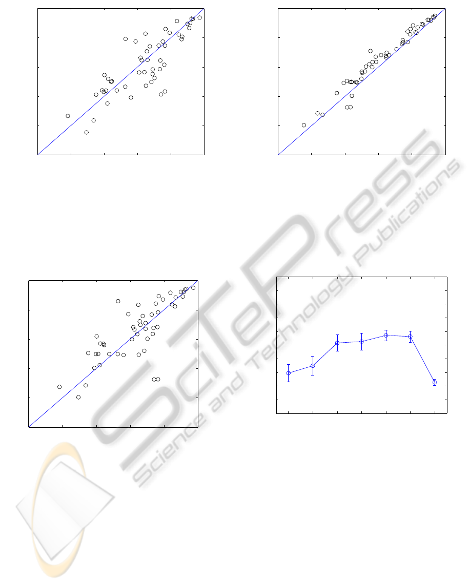
Figure 5 and Fig. 6 show a comparison of the
graph-based methods with SVMs. Out of the 50 most
common topics, SVM achieved a higher performance
than ε-Neighbourhood on 29 topics, but only beat
kNN on 19 of the topics, that is kNN performed bet-
ter than SVMs on 31 out of the 50 topics. This shows
that the graph-based methods are competitivewith the
performance of SVMs.
Figure 7 shows a comparison of the graph-based
methods. Out of the 50 most common topics, kNN has
a higher performance on 46 of the possible 50 topics.
Clearly, ε-Neighbourhood is the weaker of the graph-
based methods and so is not considered further.
ICPRAM 2012 - International Conference on Pattern Recognition Applications and Methods
30
0 20 40 60 80 100
0
20
40
60
80
100
ε−Neighbourhood F
1
Score
SVM F
1
Score
Figure 5: This figure shows a comparison of the mean
F
1
Score, averaged over all test set weeks, for ε-
Neighbourhood against SVMs on the 50 most common top-
ics. Points below the diagonal line indicate when SVMs
achieved a higher performance than ε-Neighbourhood,
with points above the diagonal line indicating that ε-
Neighbourhood achieved a higher performance than SVMs
on that topic.
0 20 40 60 80 100
0
20
40
60
80
100
SVM F
1
Score
kNN F
1
Score
Figure 6: This figure shows a comparison of the mean F
1
Score, averaged over all test set weeks, for k-NN against
SVMs on the 50 most common topics. Points below the di-
agonal line indicate when SVMs achieved a higher perfor-
mance than kNN, with points above the diagonal line indi-
cating that kNN achieved a higher performance than SVMs
on that topic.
Next, we consider the best value of µ for combin-
ing the kNN methods and SVMs in a linear combi-
nation. Figure 8 shows the performance of the com-
bined method averaged over the 50 most common top-
ics for each value of µ. Out of the 50 most common
topics, the combined method with µ = 4 provided an
improvement over the performance of both the SVM
and kNN methods for 36 of the topics. Using µ = 1
showed an improvement over both methods for the
0 20 40 60 80 100
0
20
40
60
80
100
ε−Neighbourhood F
1
Score
kNN F
1
Score
Figure 7: This figure shows a comparison of the mean F
1
Score, averaged over all test set weeks, for the graph-based
methods on the 50 most common topics. Points below the
diagonal line indicate when ε-Neighbourhood achieved a
higher performance than kNN, with points above the diago-
nal line indicating that kNN achieved a higher performance
than ε-Neighbourhood on that topic.
0 1 2 3 4 5 6
60
62
64
66
68
70
72
74
76
78
80
µ
F
1
Score
Figure 8: This figure shows a comparison of the mean F
1
Score, averaged over all test set weeks, for the combined
method at different µ values on the 50 most common topics.
It can be seen that the combined method offers an improve-
ment over the kNN approach (µ= 0) and the SVM approach
(µ = 6).
greatest number of topics, with 38 of the 50 topics
seeing an improvement. The mean performance of
the combined method with µ = 1 is lower than for
µ = 4 however, indicating that when µ = 4 the im-
provements are greater on average, even if there are
slightly fewer of them.
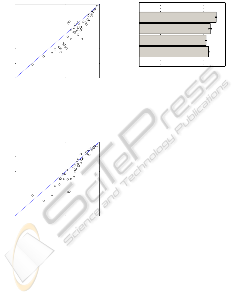
When comparingthe combined method with SVM
and kNN as seen in Fig. 9 and Fig. 10 respectively,
the performance of the combined method was higher
than SVM on 45 of the 50 topics and higher than kNN
on 41 out of the 50 topics. This shows that the com-
SCALABLE CORPUS ANNOTATION BY GRAPH CONSTRUCTION AND LABEL PROPAGATION
31
0 20 40 60 80 100
0
20
40
60
80
100
Combined Method F
1
Score
SVM F
1
Score
Figure 9: This figure shows a comparison of the mean F
1
Score, averaged over all test set weeks, for the combined
method using µ = 4 against SVMs on the 50 most com-
mon topics. Points below the diagonal line indicate when
the combined method achieved a higher performance than
SVMs, with points above the diagonal line indicating that
SVMs achieved a higher performance than the combined
method on that topic.
0 20 40 60 80 100
0
20
40
60
80
100
Combined Method F
1
Score
kNN F
1
Score
Figure 10: This figure shows a comparison of the mean
F
1
Score, averaged over all test set weeks, for the com-
bined method using µ = 4 against kNN on the 50 most
common topics. Points below the diagonal line indicate
when the combined method achieved a higher performance
than kNN, with points above the diagonal line indicating
that kNN achieved a higher performance than the combined
method on that topic.
bined method does not only improve on SVM and
kNN on average, but provides an improvement for
90% and 82% of the 50 most common topics respec-
tively. It should be noted that in the cases where the
combined method does not provide an improvement
on one of the methods, it does still have a higher per-
formance than the lowest performing method for that
topic. That is, there were no cases where combining
0 20 40 60 80
SVM
εN
kNN
Combined
Method
F
1
Score
Figure 11: This figure shows a summary of the mean F
1
Score, averaged over all test set weeks, for the graph-based
methods and SVMs along with the best combined method
(µ = 4) on the 50 most common topics. It can be seen
that the graph-based methods are comparable with SVMs,
with the combined method showing a further improvement.
It should be noted that the performance of the combined
method is slightly bias due to selecting for the best µ. ε-
Neighbourhood has been abbreviated to εN.
.
the methods gives a performance below both of the
methods individually.
A summary of the overall performance of each
method can be seen in Fig. 11. The ε-Neighbourhood
method is the weaker of the two methods proposed
with a performance of 62.2%, while the kNN method
achieved a performance of 65.9%, beating the 64.5%
for SVMs. Combining the kNN and SVM meth-
ods reached the highest performance at 71.4% with
µ = 4, showing that combining the relation-based and
content-based approaches is an effective way to im-
prove performance.
6 CONCLUSIONS
There has been an increased interest in the effects
the method of graph construction plays in the overall
performance of any graph-based approach. Findings
suggest that the method of graph construction can-
not be studied independently of the subsequent algo-
rithms applied to the graph (Maier et al., 2009). Label
propagation has many advantages over the traditional
content-based approach such as SVMs. New labels
that are introduced into the system can be adopted
with relative ease, and will automatically begin to
be propagated through the graph. In contrast, a new
SVM classifier would need to be completely trained
to classify documents with the new class label. A sec-
ond advantage of label propagation is that incorrectly
annotated documents can be reclassified based upon
new documents in a self-regulating way. That is, the
ICPRAM 2012 - International Conference on Pattern Recognition Applications and Methods
32

graph is continuously learning from new data and im-
proving its quality of annotation, while the SVM is
fixed in its classification after the initial training pe-
riod.
In this paper, we have investigated two different
local neighbourhood methods, ε-Neighbourhood and
k-Nearest Neighbour, for constructing graphs for text.
We have shown that sparse graphs can be constructed
from large text corpora in O (N logN) time, with the
cost of propagating labels on the graph linear in the
size of the graph, i.e. O (N). Our results show that the
graph-based methods are competitive with content-
based SVM methods. We have further shown that
combining the graph-based and content-based meth-
ods leads to an improvement in performance.
The proposed methods can easily be scaled out
into a distributed setting using currently available
open source software such as Apache Solr
2
, or Katta
3
,
allowing a user to handle millions of texts with simi-
larly effective performance.
Research into novel ways of combining the re-
lation and content based methods could lead to fur-
ther improvements in the categorisation performance
while keeping the cost of building and propagating la-
bels on the graph to a minimum.
ACKNOWLEDGEMENTS
I. Flaounas and N.Cristianini are supported by FP7
under grant agreement no. 231495. N. Cristianini is
supported by Royal Society Wolfson Research Merit
Award. All authors are supported by Pascal2 Network
of Excellence.
REFERENCES
Angelova, R. and Weikum, G. (2006). Graph-based text
classification: learn from your neighbors. In Proceed-
ings of the 29th annual international ACM SIGIR con-
ference on Research and development in information
retrieval, pages 485–492. ACM.
Araujo, M., Navarro, G., and Ziviani, N. (1997). Large text
searching allowing errors.
Baeza-Yates, R. and Navarro, G. (2000). Block addressing
indices for approximate text retrieval. Journal of the
American Society for Information Science, 51(1):69–
82.
Bayardo, R., Ma, Y., and Srikant, R. (2007). Scaling up
all pairs similarity search. In Proceedings of the 16th
2
Open source implementation of a distributed inverted
index. Available at: http://lucene.apache.org/solr/
3
Open source implementation of a distributed inverted
index. Available at: http://katta.sourceforge.net/
international conference on World Wide Web, pages
131–140. ACM.
Belkin, M., Matveeva, I., and Niyogi, P. (2004). Regular-
ization and semi-supervised learning on large graphs.
Learning theory, pages 624–638.
Carreira-Perpinan, M. and Zemel, R. (2004). Proximity
graphs for clustering and manifold learning. In Ad-
vances in Neural Information Processing Systems 17,
NIPS-17.
Cesa-Bianchi, N., Gentile, C., Vitale, F., and Zappella, G.
(2010a). Active learning on graphs via spanning trees.
Cesa-Bianchi, N., Gentile, C., Vitale, F., and Zappella, G.
(2010b). Random spanning trees and the prediction of
weighted graphs. In Proc. of ICML, pages 175–182.
Citeseer.
Chang, C.-C. and Lin, C.-J. (2001). LIBSVM: a library
for support vector machines. Software available at
http://www.csie.ntu.edu.tw/ cjlin/libsvm.
Cormen, T., Leiserson, C., and Rivest, R. (1990). Introduc-
tion to Algorithms.
Dietterich, T. (2000). Ensemble methods in machine learn-
ing. Multiple classifier systems, pages 1–15.
Dong, W., Moses, C., and Li, K. (2011). Efficient k-
nearest neighbor graph construction for generic sim-
ilarity measures. In Proceedings of the 20th interna-
tional conference on World wide web, pages 577–586.
ACM.
Flaounas, I., Ali, O., Turchi, M., Snowsill, T., Nicart, F., De
Bie, T., and Cristianini, N. (2011). NOAM: News Out-
lets Analysis and Monitoring System. In Proceedings
of the 2011 ACM SIGMOD international conference
on Management of data, pages 1275–1278. ACM.
Gionis, A., Indyk, P., and Motwani, R. (1999). Similarity
search in high dimensions via hashing. In Proceedings
of the 25th International Conference on Very Large
Data Bases, pages 518–529. Morgan Kaufmann Pub-
lishers Inc.
Heaps, H. (1978). Information retrieval: Computational
and theoretical aspects. Academic Press, Inc. Or-
lando, FL, USA.
Herbster, M. and Pontil, M. (2007). Prediction on a graph
with a perceptron. Advances in neural information
processing systems, 19:577.
Herbster, M., Pontil, M., and Rojas-Galeano, S.(2009). Fast
prediction on a tree. Advances in Neural Information
Processing Systems, 21:657–664.
Jebara, T., Wang, J., and Chang, S. (2009). Graph construc-
tion and b-matching for semi-supervised learning. In
Proceedings of the 26th Annual International Confer-
ence on Machine Learning, pages 441–448. ACM.
Joachims, T. (1998). Text categorization with support vec-
tor machines: Learning with many relevant features.
Machine Learning: ECML-98, pages 137–142.
Lewis, D., Yang, Y., Rose, T., and Li, F. (2004). RCV1:
A new benchmark collection for text categorization
research. Journal of Machine Learning Research,
5:361–397.
Lloyd, L., Kechagias, D., and Skiena, S. (2005). Lydia: A
system for large-scale news analysis. In String Pro-
cessing and Information Retrieval, pages 161–166.
Springer.
SCALABLE CORPUS ANNOTATION BY GRAPH CONSTRUCTION AND LABEL PROPAGATION
33

Maier, M., Von Luxburg, U., and Hein, M. (2009). Influ-
ence of graph construction on graph-based clustering
measures. Advances in neural information processing
systems, 22:1025–1032.
Parzen, E. (1962). On estimation of a probability density
function and mode. The annals of mathematical statis-
tics, 33(3):1065–1076.
Salton, G. (1989). Automatic text processing.
Sarawagi, S. and Kirpal, A. (2004). Efficient set joins on
similarity predicates. In Proceedings of the 2004 ACM
SIGMOD international conference on Management of
data, pages 743–754. ACM.
Sebastiani, F. (2002). Machine learning in automated
text categorization. ACM computing surveys (CSUR),
34(1):1–47.
Shawe-Taylor, J. and Cristianini, N. (2004). Kernel methods
for pattern analysis. Cambridge University Press.
Steinbach, M., Karypis, G., and Kumar, V. (2000). A com-
parison of document clustering techniques. In KDD
workshop on text mining, volume 400, pages 525–526.
Citeseer.
Steinberger, R., Pouliquen, B., and van der Goot, E. (2009).
An Introduction to the Europe Media Monitor Family
of Applications. In Information Access in a Multilin-
gual World-Proceedings of the SIGIR 2009 Workshop,
pages 1–8.
Tan, P., Steinbach, M., Kumar, V., et al. (2006). Introduction
to data mining. Pearson Addison Wesley Boston.
Yang, Y., Zhang, J., and Kisiel, B. (2003). A scalability
analysis of classifiers in text categorization. In Pro-
ceedings of the 26th annual international ACM SI-
GIR conference on Research and development in in-
formaion retrieval, pages 96–103. ACM.
Zhang, J., Marszałek, M., Lazebnik, S., and Schmid, C.
(2007). Local Features and Kernels for Classifica-
tion of Texture and Object Categories: A Comprehen-
sive Study. International Journal of Computer Vision,
73(2):213–238.
Zhu, X. (2007). Semi-supervised learning literature survey.
Computer Science, University of Wisconsin-Madison.
Zhu, X., Ghahramani, Z., and Lafferty, J. (2003). Semi-
supervised learning using gaussian fields and har-
monic functions. In International Conference of Ma-
chine Learning, volume 20, page 912.
ICPRAM 2012 - International Conference on Pattern Recognition Applications and Methods
34
