
WHAT DO OBJECTS FEEL LIKE?
Active Perception for a Humanoid Robot
Jens Kleesiek
1,3
, Stephanie Badde
2
, Stefan Wermter
3
and Andreas K. Engel
1
1
Dept. of Neurophysiology and Pathophysiology, University Medical Center Hamburg-Eppendorf, Hamburg, Germany
2
Dept. of Biological Psychology and Neuropsychology, University of Hamburg, Hamburg, Germany
3
Department of Informatics, Knowledge Technology, University of Hamburg, Hamburg, Germany
Keywords:
Active perception, RNNPB, Humanoid robot.
Abstract:
We present a recurrent neural architecture with parametric bias for actively perceiving objects. A humanoid
robot learns to extract sensorimotor laws and based on those to classify eight objects by exploring their multi-
modal sensory characteristics. The network is either trained with prototype sequences for all objects or just two
objects. In both cases the network is able to self-organize the parametric bias space into clusters representing
individual objects and due to that, discriminates all eight categories with a very low error rate. We show that
the network is able to retrieve stored sensory sequences with a high accuracy. Furthermore, trained with only
two objects it is still able to generate fairly accurate sensory predictions for unseen objects. In addition, the
approach proves to be very robust against noise.
1 INTRODUCTION
The active nature of perception and the intimate re-
lation between action and cognition (Dewey, 1896;
Merleau-Ponty, 1963) has been emphasized in philos-
ophy and cognitive science for a long time. “Percep-
tion is something you do, not something that happens
to you” (Bridgeman and Tseng, 2011) has been postu-
lated in the neurosciences as well as in related fields.
Already in the 80’s of the last century it has been sug-
gested for machine perception and robotics that “[. . . ]
it should be axiomatic that perception is not passive,
but active. Perceptual activity is exploratory, prob-
ing, searching; percepts do not simply fall onto sen-
sors as rain falls onto ground. We do not just see, we
look” (Bajcsy, 1988). However, most of the current
approaches do not follow these insights.
In the computer vision and robotics literature ex-
pressions like ’active vision’ (Aloimonos et al., 1988),
’active perception’ (Bajcsy, 1988), ’smart sensing’
(Burt, 1988) and ’animate vision’ (Ballard, 1991) are
commonly used – sometimes even interchangeably,
despite varying intentions pursued by the original au-
thors. Usually, these terms refer to a sensor, which
can be moved actively, e. g. a scanning laser mounted
on an autonomous vehicle travelling offroad at high
speed (Patel et al., 2005) or a four-camera stereo head
using foveation for detection and fixation of objects
(Rasolzadeh et al., 2009). The mobility of a sensor or
of a manipulator, e. g. robot arm, and especially the
knowledge about the movements in conjunction with
a changing sensory impression have been proven to be
of valuable assistance for object segmentation (Fitz-
patrick and Metta, 2003).
We take the notion of active perception a step fur-
ther and do not restrict it to the visual modality only.
Varela et al. suggested an enactive approach – mean-
ing that cognitive behavior results from interaction
of organisms with their environment (Varela et al.,
1991). A robot is embodied (Pfeifer et al., 2007) and
it has the ability to act and to perceive. In our opin-
ion it actually needs to act to perceive. The action-
triggered sensations are guided by the physical prop-
erties of its body, the world and the interplay of both.
Here we propose a model that can be seen as a first
step towards this meaning of active perception. A hu-
manoid robot moves toy bricks up-and-down and ro-
tates them back-and-forth, while holding them in its
hand. The induced multi-modal sensory impressions
are used to train an improved version of a recurrent
neural network with parametric bias (RNNPB), origi-
nally developed by Tani et al. (Tani and Ito, 2003). As
a result, the robot is able to self-organize the contex-
tual information to sensorimotor laws, which in turn
can be used for object classification. Due to the over-
whelming generalization capabilities of the recurrent
64
Kleesiek J., Badde S., Wermter S. and K. Engel A..
WHAT DO OBJECTS FEEL LIKE? - Active Perception for a Humanoid Robot.
DOI: 10.5220/0003729900640073
In Proceedings of the 4th International Conference on Agents and Artificial Intelligence (ICAART-2012), pages 64-73
ISBN: 978-989-8425-95-9
Copyright
c
2012 SCITEPRESS (Science and Technology Publications, Lda.)

architecture, the robot is even able to correctly clas-
sify unknown objects. Furthermore, we show that the
proposed model is very robust against noise.
The paper is organized as follows. In section 2
we present the neural architecture, followed by a task,
scenario and data description in section 3. Then we
report on three experiments in section 4, concluding
with a discussion of the results, the architecture and
related literature in section 5.
2 RECURRENT NEURAL
NETWORK
Despite its intriguing properties the recurrent neural
network with parametric bias has hardly been used by
others than the original authors. Mostly, the archi-
tecture is utilized to model the mirror neuron system
(Tani et al., 2004; Cuijpers et al., 2009). Here we
apply the variant proposed by Cuijpers et al. using
an Elman-type structure at its core (Cuijpers et al.,
2009). Furthermore, we modify the training algo-
rithm to include adaptive learning rates for training
of the weights as well as the PB values. This results
in an improved architecture that is more stable and
converges faster. For instance, the storage of two 1-D
time series (t = 12) is sped up by a factor of 22 on
average (n = 1000, 5519 vs. 122.709 steps).
2.1 Storage of Time Series
The recurrent neural network with parametric bias
(an overview of the architecture unfolded in time can
be seen in Fig. 1) can be used for the storage, re-
trieval and recognition of sequences. For this pur-
pose, the parametric bias (PB) vector is learned si-
multaneously and unsupervised during normal train-
ing of the network. The prediction error with re-
spect to the desired output is determined and back-
propagated through time (BPTT) (Kolen and Kremer,
2001). However, the error is not only used to correct
all the synaptic weights present in an Elman-type net-
work. Additionally, the error with respect to the PB
nodes δ
PB
is accumulated over time and used for up-
dating the PB values after an entire forward-backward
pass of a single time series, denoted as epoch e. In
contrast to the synaptic weights that are shared by all
training patterns, a unique PB vector is assigned to
each individual training sequence. The update equa-
tions for the i-th unit of the parametric bias pb for a
time series of length T is given as:
ρ
i
(e + 1) = ρ
i
(e) + γ
i
T
∑
t=1
δ
PB
i,t
, (1)
pb
i
(e) = sigmoid(ρ
i
(e)) , (2)
where γ is the update rate for the PB values, which in
contrast to the original version is during training not
constant and not identical for every PB unit. Instead,
it is scaled proportional to the absolute mean value
of prediction errors being backpropagated to the i-th
node over time T :
γ
i
∝
1
T
T
∑
t=1
δ
PB
i,t
. (3)
The other adjustable weights of the network are up-
dated via an adaptive mechanism, inspired by the re-
silient propagation algorithm (Riedmiller and Braun,
1993). However, there are decisive differences. First,
the learning rate of each neuron is adjusted after every
epoch. Second, not the sign of the partial derivative
of the corresponding weight is used for changing its
value, but instead the partial derivative itself is taken.
To determine if the partial derivative of weight w
i j
changes its sign we can compute:
ε
i j
=
∂E
i j
∂w
i j
(t − 1) ·
∂E
i j
∂w
i j
(t) (4)
If ε
i j
< 0 the last update was too big and the local
minimum has been missed. Therefore, the learning
rate η
i j
has to be decreased by a factor ξ
−
< 1 . On
the other hand a positive derivative indicates that the
learning rate can be increased by a factor ξ
+
> 1 to
speed up convergence. This update of the learning
rate can be formalized as:
η
i j
(t) =
max(η
i j
(t − 1) · ξ
−
, η
min
) if ε
i j
< 0,
min(η
i j
(t − 1) · ξ
+
, η
max
) if ε
i j
> 0,
η
i j
(t − 1) else.
(5)
The succeeding weight update ∆w
i j
then obeys the
following rule:
∆w
i j
(t) =
(
−∆w
i j
(t − 1) if ε
i j
< 0,
η
i j
(t) ·
∂E
i j
∂w
i j
(t) else.
(6)
In addition to reverting the previous weight change in
the case of ε
i j
< 0 the partial derivative is also set to
zero (
∂E
i j
∂w
i j
(t) = 0). This prevents changing of the sign
of the derivative once again in the succeeding step and
thus a potential double punishment.
We use a nonlinear activation function with rec-
ommended parameters (LeCun et al., 1998) for all
neurons in the network as well as for the PB units
(Eq. 2):
sigmoid(x) = 1.7159 · tanh
2
3
· x
. (7)
WHAT DO OBJECTS FEEL LIKE? - Active Perception for a Humanoid Robot
65
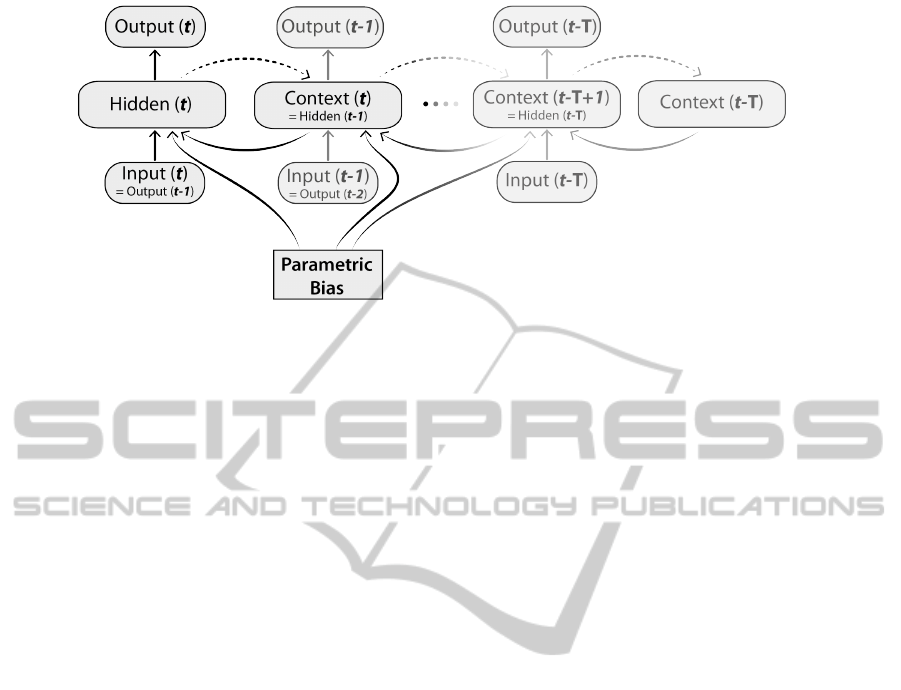
Figure 1: Network architecture. The Elman-type Recurrent Neural Network with Parametric Bias (RNNPB) unfolded in
time. Dashed arrows indicate a verbatim copy of the activations (weight connections set equal to 1.0). All other adjacent
layers are fully connected. t is the current time step, T denotes the length of the time series.
2.2 Number of PB Units
The PB vector is usually low dimensional and resem-
bles bifurcation parameters of a nonlinear dynamical
system, i. e. it characterizes fixed-point dynamics of
the RNN. To quantify the number of the principle
components (PCs) actually needed for (almost) loss-
less reconstruction of the PB space, we determined
how many are necessary to explain 99 % of the vari-
ance. Increasing the number of PB values, given a
bi-modal time series of length T = 14, resulted in a
constant number of two PCs. Hence, we use a 2-D
PB vector for our experiments.
2.3 Retrieval
During training the PB values are self-organized,
thereby encoding each time series and arranging it
in PB space according to the properties of the train-
ing pattern. This means that the values of similar
sequences are clustered together, whereas more dis-
tinguishable ones are located further apart. Once
learned, the PB values can be used for the genera-
tion of the time series previously stored. For this pur-
pose, the network is operated in closed-loop mode.
The PB values are ’clamped’ to a previously learned
value and the forward pass of the network is executed
from an initial input I(0). In the next time steps, the
output at time t serves as an input at time t + 1. This
leads to a reconstruction of the training sequence with
a very high accuracy, only limited by the convergence
threshold used during learning (e. g. shown in Fig. 5
on the left).
2.4 Recognition
A previously stored (time) sequence can also be rec-
ognized via its corresponding PB value. Therefore,
the observed sequence is fed into the network without
updating any connection weights. Only the PB values
are accumulated according to Eq. (1) and (2) using a
constant learning rate γ this time. Once a stable PB
vector is reached (as shown in Fig. 6), it can be com-
pared to the one obtained during training.
2.5 Generalized Recognition and
Generation
The network has substantial generalization potential.
Not only previously stored sequences can be recon-
structed and recognized. But, (time) sequences apart
from the stored patterns can be generated. Since only
the PB values but not the synaptic weights are updated
in recogniton mode, a stable PB value can also be as-
signed to an unknown sequence.
For instance, training the network with two sine
waves of different frequencies allows to generate
cyclic functions with intermediate frequencies sim-
ply by operating the network in generation mode and
varying the PB values within the interval of the PB
values obtained during training. Furthermore, the PB
values obtained during recognition of a previously
unseen sine function with an intermediate frequency,
w. r. t. the training sequences, will lie within the range
of the PB values acquired during learning. Hence, the
network is able to capture a reciprocal relationship be-
tween a time series and its associated PB value.
ICAART 2012 - International Conference on Agents and Artificial Intelligence
66

2.6 Network Parameters
Based on systematic empirical trials, the following
parameters have been determined for our experi-
ments. The network contained two input and two out-
put nodes, 24 hidden and 24 context neurons as well
as 2 PB units (cf. section 2.2). The convergence crite-
rion for BPTT was set to 10
−6
in the first, and 10
−5
in
the second experiment. For recognition of a sequence
the update rate γ of the PB values was set to 0.1.
The values for all other individual adaptive learning
rates (Eq. 5) during training of the synaptic weights
were allowed to be in the range of η
min
= 10
−12
and
η
max
= 50; depending on the gradient they were ei-
ther increased with ξ
+
= 1.01 or decreased by a factor
ξ
−
= 0.9.
3 SCENARIO
The humanoid robot Nao from Aldebaran Robotics
(http://www.aldebaran-robotics.com/) is pro-
grammed to conduct the experiments (Fig. 2a). The
task for the robot is to identify what object (toy brick)
it holds in its hand. In total there are eight object cat-
egories that have to be distinguished by the robot: the
toy bricks have four different shapes (circular-, star-
, rectangular- and triangular-shaped), which exist in
two different weight versions (light and heavy) each.
Hence, for achieving a successful classification multi-
modal sensory impressions are required. Addition-
ally, active perception is necessary to induce sensory
changes essential for discrimination of, depending on
the perspective, similar looking shapes, e. g. star- and
circular-shaped objects. For this purpose, the robot
performs a predefined motor sequence and simultane-
ously acquires visual and proprioceptive sensor val-
ues.
3.1 Data Acquisition
The recorded time series comprises 14 sensor values
for each modality. In each single trial the robot turns
its wrist with the object between its fingers by 45.8
◦
back-and-forth twice, followed by lifting the object
up-and-down three times (thereby altering the pitch
of the shoulder joint by 11.5
◦
) and finally, turning it
again twice.
After an action has been completed the raw im-
age of the lower camera of the Nao robot is cap-
tured, whereas the electric current of the shoulder
pitch servo motor is recorded constantly (sampling
frequency 10 hz) over the entire movement interval.
For each object category 10 single trial time series are
Figure 2: Scenario. a) Toy bricks in front of the humanoid
robot Nao. The toy bricks exist in four different shapes,
have an identical color and are either light-weight (15 g)
or heavy (50 g). This results in a total of eight categories
that have to be distinguished by the robot. b) Rotation
movement with the star-shaped object captured by the robot
camera. In the upper row the raw camera image is shown,
whereas the bottom row depicts the preprocessed image that
is used to compute the visual feature.
recorded in the described way and processed in real-
time. This yields 80 bi-modal time series in total.
3.2 Data Processing
For the proprioceptive measurements only the mean
values are computed for the time intervals lying in-
between movements. The visual processing, on the
other hand, involves several steps (Fig. 2b), which
are accomplished by using OpenCV (Bradski, 2000).
First, the raw color image is converted to a binary im-
age using a color threshold. Next, the convex hull is
computed and, based on that, the contour belonging
to the toy brick is extracted (Suzuki and Be, 1985).
For the identified contour the first Hu moment h
1
is
calculated (Hu, 1962) by combining the normalized
central moments η
pq
linearly.
η
pq
=
µ
pq
µ
p+q
2
+1
00
, (8)
h
1
= η
20
+ η
02
. (9)
As a particular feature the Hu moments are scale,
translation and rotation invariant. Finally, the vi-
sual measurements are scaled to be in the interval
[−0.5, 0.5].
We are aware that more discriminative geometri-
cal features exist, e. g. orthogonal variant moments
(Mart
´
ın H. et al., 2010). However, we deliberately
posed the problem this way to make it a challenging
task and show the potential of the approach.
3.3 Training and Test Data
For testing, the data of single trials is used, i. e. 10
2-D time series per object category (one dimension
WHAT DO OBJECTS FEEL LIKE? - Active Perception for a Humanoid Robot
67
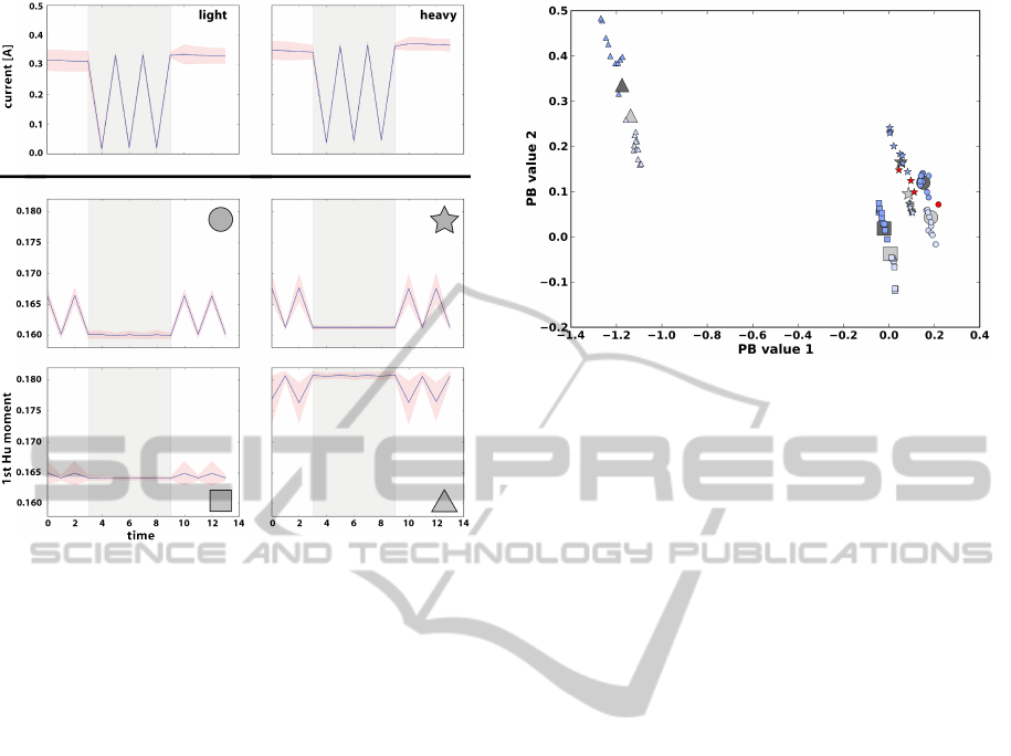
Figure 3: Training data. The mean values of the two
weight conditions (light and heavy, top) and the four vi-
sual conditions (matching symbols, bottom) are shown.
These mean time series are used as prototypes for training
of the RNNPB. Gray shaded area represents the up-and-
down movement, whereas back-and-forth movements are
unshaded. The red area surrounding the signals delineates
two standard deviations from the mean.
for each modality). However, for training a proto-
type for each object category and modality is deter-
mined (Fig. 3). To obtain this subclass representative,
the mean value of pooled single trials, with regard to
identical object properties, is computed. This means
that for instance all circular-shaped objects are com-
bined (n = 20) and used to compute the visual pro-
totype for circular-shaped objects. To find the pro-
prioceptive prototype for e. g. all heavy objects, all
individual measurements with this property (n = 40)
are aggregated and used to calculate the mean value
at each time step. The subclass prototypes are then
combined to form a 2-D multi-modal time series that
serves as an input for the recurrent neural network
during training.
4 RESULTS
4.1 Experiment 1 – Classification using
All Object Categories for Training
Three experiments have been conducted. In the first
Figure 4: Experiment 1 – Classification using all object
categories for training. PB values of the class prototypes
used for training are depicted in light and dark gray and
with a symbol matching the corresponding shape. Smaller
symbols depict PB values obtained during testing with bi-
modal single trial data. If the objects have been correctly
classified they are shown in light or dark blue, otherwise in
red. Light colors are used for light-weight, dark colors for
heavy-weight objects.
experiment the improved recurrent neural network
with parametric bias is trained with the bi-modal pro-
totype time series of all eight object categories (see
Fig. 3 and section 3.3). During training, the PB val-
ues for the respective categories emerge in an unsu-
pervised way. This means, the two-dimensional PB
space is self-organized based on the inherent proper-
ties of the sensory data that is presented to the net-
work. Hence, objects with similar dynamic sensory
properties are clustered together. This can be seen
in Fig. 4. For instance, the learned PB vectors repre-
senting star- and circular-shaped objects, either light-
weight (light gray) or heavy (dark gray), are located in
close proximity, whereas the PB values coding for the
triangular-shaped objects are positioned more distant.
This is due to the deviating visual sensory impression
they generate (Fig. 3). The experiment has been re-
peated several times with different random initializa-
tions of the network weights. However, the obtained
PB values of the different classes always demonstrate
a comparable geometric relation with respect to each
other.
To demonstrate the retrieval properties (section
2.3) of the fully trained architecture the PB values ac-
quired during training are ’clamped’ to the network.
Operating the network in closed-loop shows that the
input sequences used for training can be retrieved
with a very high accuracy. This is as an example
shown in Fig. 5 (left) for the heavy star-shaped object.
The steps needed until stable PB values are
reached, which in turn can be used for recognition, are
ICAART 2012 - International Conference on Agents and Artificial Intelligence
68
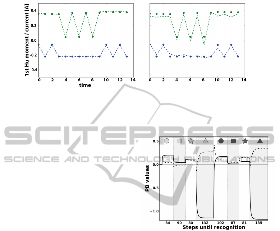
Figure 5: Retrieval and generation capabilities. Proprioceptive (green) and visual (blue) dots represent the sampling points
of the heavy star-shaped prototype time series (Fig. 3). Dashed lines are the time series generated by the network operated in
closed-loop with ’clamped’ PB values as the only input. The PB values have been acquired unsupervised either during full
training (left) or partial training (right). During partial training (right) the network has only been trained with the prototype
sequences for the light-weight circle and the heavy triangle. Still, the network is able to generate a fairly accurate sensory
prediction for the (untrained) heavy star-shaped object.
illustrated in Fig. 6. The bi-modal sensory sequences
for all light-weight and heavy objects are fed consec-
utively into the network. On average it takes less than
100 steps (about 200 ms) until the PB values have con-
verged. The convergence criterion is set to 20 consec-
utive iterations where the cumulative change of both
PB values is < 10
−5
. To assure that the PB values
reached a stable state, this number was successfully
increased to 100.000 consecutive steps in preliminary
experiments (not shown). Note, that the network and
PB values are not re-initialized when the next sensory
sequence is presented to the network. Thus, the robot
can continuously interact with the toy bricks and is
able to immediately recognize an object based on its
sensorimotor sequence.
For testing, the network is operated in general-
ized recognition mode (section 2.5). Single trial bi-
modal sensory sequences are presented to the network
that in turn provides an ’identifying’ PB value. The
class membership, i. e. which object the robot holds
in its hand and how heavy this object is, is then deter-
mined based on the minimal Euclidean distance to the
PB values of the class prototypes (gray symbols). In
Fig. 4 the PB values of all 80 single trial test patterns
are depicted.
Only 4 out of 80 objects are misclassified (shown
in red), yielding an error rate of 5 %. Interestingly,
only star- and circular-shaped objects are confused by
the network, which indeed generate very similar sen-
sory impressions (Fig. 3). To assess the meaning of
the error rate and estimate how challenging the posed
problem is, we evaluate the data with two other com-
monly used techniques in machine learning. First, we
train a multi-layer perceptron (28 input, 14 hidden and
one output unit) with the prototype sequences. Test-
ing with the single trial data results in an error rate
Figure 6: Steps until stable PB values are reached. Bi-
modal sensory sequences for all light-weight and heavy ob-
jects (represented by matching symbols in light and dark
gray, respectively) are consecutively fed into the network.
The time courses of PB value 1 (solid line) and PB value 2
(dashed line) during the recognition process are plotted.
of 46.8 %, reflecting weaker generalization capabili-
ties of the non-recurrent architecture. Next, we train
and evaluate our data with a support vector classi-
fier (SVC) using default parameters (Chang and Lin,
2011). In contrast, this method is able to classify the
data perfectly.
4.2 Experiment 2 – Classification using
Only the Light Circular-shaped and
the Heavy Triangular-shaped
Object for Training
In experiment 2 only the bi-modal prototypes for the
light circular- and heavy triangular-shaped objects are
used to train the RNNPB. Although, the absolute PB
WHAT DO OBJECTS FEEL LIKE? - Active Perception for a Humanoid Robot
69
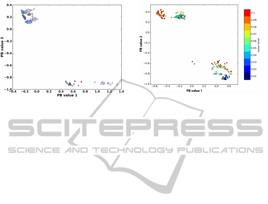
Figure 7: Experiment 2 – Classification using only the
light circular-shaped and the heavy triangular-shaped
object for training. PB values of the class prototypes used
for training are depicted in light and dark gray and with a
symbol matching the corresponding shape. The a posteri-
ori computed cluster centers of the untrained object cate-
gories are depicted using larger symbols in either light or
dark blue. Smaller symbols are used for PB values of sen-
sory data of single trials. If the objects have been correctly
classified they are shown in light or dark blue, otherwise in
red. Light colors are used for light-weight, dark colors for
heavy-weight objects.
values obtained during training differ from the ones
being determined in the previous experiment, their
relative Euclidean distance in PB space is nearly the
same (1.39 vs. 1.35), stressing the data-driven self-
organization of the parametric bias space.
For testing, initially only the bi-modal sensory
time series matching the two training conditions are
fed into the network, thereby determining their PB
values. Using the Euclidean distance subsequently to
obtain the class membership results in a flawless iden-
tification of the two categories.
Further evaluation of the single trial test data is
performed in two stages. In a primary step the remain-
ing test data is presented to the network and the re-
spective PB values are computed (generalized recog-
nition, section 2.5). Despite not having been trained
with prototypes for these six object categories, the
network is able to clusters PB values stemming from
similar sensory situations, i. e. identical object cate-
gories. In a succeeding step we compute the centroid
for each class (mean PB value) and classify again
based on the Euclidean distance. This time only two
single trial time series are misclassified by the net-
work (error rate 2.5 %). The results are shown in
Fig. 7.
The generalization potential (section 2.5) of the
architecture is presented in Fig. 5 (right) for the heavy
star-shaped object. For this purpose, the mean PB val-
ues (centroid of the respective class) are clamped to
Figure 8: Uni-modal noise tolerance. Uniformly dis-
tributed noise of increasing levels (color coded) is only
added to the visual prototype time series for the light-weight
circle and the heavy triangle. The PB values are determined
and marked with a matching symbol.The light gray circle
and dark gray triangle show the PB values obtained during
training without noise.
the network, which is operated in closed-loop mode.
The network has only been trained with the light
circular- and the heavy triangular-shaped object. Still,
it is possible to generate sensory predictions for un-
seen objects, e. g. the heavy star-shaped toy brick, that
match fairly well the real sensory impressions.
4.3 Experiment 3 – Noise Tolerance
within and Across Modalities
Based on the network weights that have been ob-
tained in experiment 2 (training the RNNPB only
with the bi-modal prototypes for the light circular-
and heavy triangular-shaped objects), we evaluate the
noise tolerance of the recurrent neural architecture.
For this purpose, uniformly distributed noise of in-
creasing levels is either added to the visual prototype
time series only (Fig. 8) or to the time series of both
modalities (Fig. 9).
As it can be seen for both conditions, even high
levels of noise allow for a reliable linear discrimina-
tion of the two classes. Furthermore, the PB values
of increasing noise levels show commonalities and
are clustered together, again providing evidence for
a data-driven self-organization of the PB space. Thus,
determining the Euclidean distance of the PB values
obtained from the noisy signals to the class represen-
tatives enables not only to determine the class mem-
bership, it also allows to estimate the noise level with
respect to the prototypical sensory impression.
ICAART 2012 - International Conference on Agents and Artificial Intelligence
70
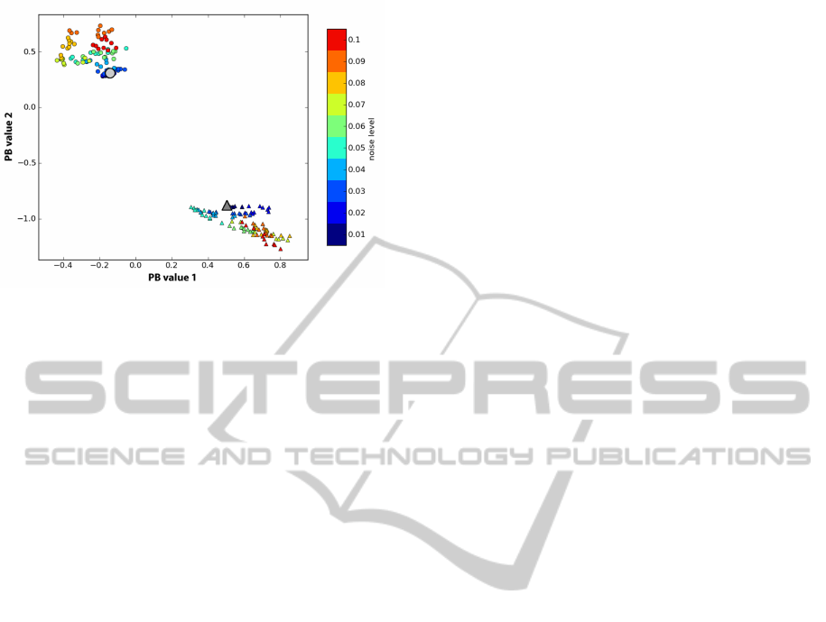
Figure 9: Bi-modal noise tolerance. Uniformly distributed
noise of increasing levels (color coded) is added to both (vi-
sual and proprioceptive) prototype time series for the light-
weight circle and the heavy triangle. The PB values are
determined and marked with a matching symbol. The light
gray circle and dark gray triangle show the PB values ob-
tained during training without noise.
5 DISCUSSION
We present a robust model with low error rates for
object classification on a real humanoid robot. How-
ever, our primary goal is not to compete with other
approaches used for object classification. Instead,
our intention is to provide a neuroscientifically and
philosophically inspired model for what do objects
feel like? For this purpose, we stress the active na-
ture of perception within and across modalities. Ac-
cording to the theory of sensorimotor contingencies
(SMCs), proposed by O’Regan and No
¨
e, actions are
fundamental for perception and help to distinguish the
qualities of sensory experiences in different sensory
channels, e. g. ’seeing’ or ’touching’ (O’Regan and
No
¨
e, 2001). It is suggested that “seeing is a way of
acting”. Exactly this is mimicked in our experiments.
A motor sequence induces multi-modal sensory
changes. During learning these high-dimensional per-
ceptions are ’engraved’ in the network. Simultane-
ously, low-dimensional PB values emerge unsuper-
vised, coding for a sensorimotor sequence character-
izing the interplay of the robot with an object. We
show that 2-D time series of length T = 14 can be reli-
ably represented by a 2-D PB vector and that this vec-
tor allows to recall learned sensory sequences with a
high accuracy (Fig. 5 left). Furthermore, the geomet-
rical relation of PB vectors of different objects can
be used to infer relations between the original high
dimensional time series, e. g. the sensation of a star-
shaped object ’feels’ more like a circular-shaped ob-
ject than a triangular-shaped one. Due to the exper-
imental noise of single trials, identical objects cause
varying sensory impressions. Still, the RNNPB can
be used to recognize those (Fig. 4). Additionally, sen-
sations belonging to unknown objects can be discrim-
inated from known (learned) ones. Moreover, sensa-
tions arising from different unknown objects can be
kept apart from each other reliably (Fig. 7).
Humans are able to immediately divide the per-
ceived world into different physical objects, seem-
ingly without effort, even when they are confronted
with previously unseen objects. Indeed, it makes per-
fect sense that the discrimination between different
sensory qualia is possible without training (section
4.2). However, actively generating (retrieving) sen-
sorimotor experiences does require training and gen-
eralization capabilities. Similar findings have been re-
ported recently for humans (Held et al., 2011). Pre-
viously blind subjects, regaining sight after a surgical
procedure, were able to visually discriminate different
objects right away. Cross-modal mappings between
seen and felt, however, had to be learned.
Comparing the classification results of the fully
trained RNNPB with the SVC reveals a superior per-
formance of the support vector classifier. Neverthe-
less, it has to be kept in mind that the maximum mar-
gin classifier cannot be used to generate or retrieve
time series. Interestingly, the error rate is lower if the
recurrent network is only trained with two object cate-
gories (section 4.2). A potential explanation, besides
random fluctuations, could be that during training a
common set of weights has to be found for all object
categories. This process presumably interferes, due to
the challenging input data, with the self-organization
of the PB space.
A drawback of the presented model is that it
currently operates on a fixed motor sequence. It
would be desirable if the robot performs motor bab-
bling (Olsson et al., 2006) leading not only to a
self-organization of the sensory space, but to a self-
organization of the sensorimotor space. A simple so-
lution to this problem would be to train the network
additionally with the motor sequence most appropri-
ate for an object, i. e. reflecting its affordance (Gibson,
1977). This would lead to an even better classifica-
tion result, because the motor sequences themselves
would help to distinguish the objects from each other
and thus the emerging PB values would be arranged
further apart in PB space. Conversely, this means cur-
rently it does not make sense to train the network with
the identical motor sequences in addition. However,
that does not address that the robot should identify the
object affordances, the movements characterizing an
object, by itself. Further lines of research will specif-
ically address this issue.
WHAT DO OBJECTS FEEL LIKE? - Active Perception for a Humanoid Robot
71

In related research, Ogata et al. also extract multi-
modal dynamic features of objects, while a humanoid
robot interacts with them (Ogata et al., 2005). How-
ever, there are distinct differences. Despite using
fewer objects in total, the problem posed in our ex-
periments is considerably harder. Our toy bricks have
approximately the same circumference and identical
color. Furthermore, they exist in two weight classes
with an identical in-class weight that can only be dis-
criminated via multi-modal sensory information. We
provide classification results, compare the results to
other methods (MLP and SVC) and evaluate the noise
tolerance of the architecture. In addition, we only use
prototype time series for training (in contrast to using
all single trial time series) resulting in a reduced train-
ing time. Further, we demonstrate that, if the network
has already learned sensorimotor laws of certain ob-
jects, it is able to generalize and provide fairly accu-
rate sensory predictions for unseen ones (Fig. 5 right).
In conclusion, we present a promising framework
for object classification based on active perception on
a humanoid robot, rooted in neuroscientific and philo-
sophical hypotheses.
5.1 Future Work
There are several potential applications of the pre-
sented model. As shown in Fig. 8 and 9 the network
tolerates noise very well. This fact can be used for
sensor de-noising. Despite receiving a noisy sensory
signal, the robot will still be able to determine the PB
values of the class representative based on the Eu-
clidean distance. In turn, these values can be used
to operate the RNNPB in retrieval mode (section 2.3)
generating the noise-free sensory signal previously
stored, which then can be processed further. It is also
conceivable, that the network is used for sensory (sen-
sorimotor) imagery. Due to the powerful generaliza-
tion capabilities of the network not only the trained
sensory perceptions can be recalled, but interpolated
’feelings’ can be generated (Fig. 5 right).
ACKNOWLEDGEMENTS
This work was supported by the Sino-German Re-
search Training Group CINACS, DFG GRK 1247/1
and 1247/2, and by the EU projects KSERA under
2010-248085. We thank R. Cuijpers and C. Weber
for inspiring and very helpful discussions, S. Hein-
rich, D. Jessen and N. Navarro for assistance with the
robot.
REFERENCES
Aloimonos, J., Weiss, I., and Bandyopadhyay, A. (1988).
Active vision. International Journal of Computer Vi-
sion, 1:333–356.
Bajcsy, R. (1988). Active perception. Proceedings of the
IEEE, 76(8):966 –1005.
Ballard, D. H. (1991). Animate vision. Artificial Intelli-
gence, 48(1):57–86.
Bradski, G. (2000). The OpenCV Library. Dr. Dobb’s Jour-
nal of Software Tools.
Bridgeman, B. and Tseng, P. (2011). Embodied cogni-
tion and the perception-action link. Phys Life Rev,
8(1):73–85.
Burt, P. (1988). Smart sensing within a pyramid vision ma-
chine. Proceedings of the IEEE, 76(8):1006 –1015.
Chang, C.-C. and Lin, C.-J. (2011). LIBSVM: A library
for support vector machines. ACM Transactions on
Intelligent Systems and Technology, 2:27:1–27:27.
Cuijpers, R. H., Stuijt, F., and Sprinkhuizen-Kuyper, I. G.
(2009). Generalisation of action sequences in RN-
NPB networks with mirror properties. In Proceedings
of the 17th European symposium on Artifical Neural
Networks (ESANN), pages 251–256.
Dewey, J. (1896). The reflex arc concept in psychology.
Psychological Review, 3:357–370.
Fitzpatrick, P. and Metta, G. (2003). Grounding vision
through experimental manipulation. Philosophical
Transactions of the Royal Society of London. Series
A: Mathematical, Physical and Engineering Sciences,
361(1811):2165–2185.
Gibson, J. J. (1977). The theory of affordances. In Shaw,
R. and Bransford, J., editors, Perceiving, acting, and
knowing: Toward an ecological psychology, pages
67–82. Hillsdale, NJ: Erlbaum.
Held, R., Ostrovsky, Y., Degelder, B., Gandhi, T., Ganesh,
S., Mathur, U., and Sinha, P. (2011). The newly
sighted fail to match seen with felt. Nat Neurosci,
14(5):551–3.
Hu, M.-K. (1962). Visual pattern recognition by moment
invariants. Information Theory, IRE Transactions on,
8(2):179 –187.
Kolen, J. F. and Kremer, S. C. (2001). A field guide to dy-
namical recurrent networks. IEEE Press, New York.
LeCun, Y., Bottou, L., Orr, G., and M
¨
uller, K. (1998). Ef-
ficient backprop. Lecture Notes in Computer Science,
1524:5–50.
Mart
´
ın H., J. A., Santos, M., and de Lope, J. (2010). Or-
thogonal variant moments features in image analysis.
Inf. Sci., 180:846–860.
Merleau-Ponty, M. (1963). The structure of behavior. Bea-
con Press, Boston.
Ogata, T., Ohba, H., Tani, J., Komatani, K., and Okuno,
H. G. (2005). Extracting multi-modal dynamics of ob-
jects using RNNPB. Proc. IEEE/RSJ Int. Conf. on In-
telligent Robots and Systems, Edmonton, pages 160–
165.
Olsson, L. A., Nehaniv, C. L., and Polani, D. (2006). From
unknown sensors and actuators to actions grounded
in sensorimotor perceptions. Connection Science,
18(2):121–144.
ICAART 2012 - International Conference on Agents and Artificial Intelligence
72

O’Regan, J. K. and No
¨
e, A. (2001). A sensorimotor account
of vision and visual consciousness. Behav Brain Sci,
24(5):939–73; discussion 973–1031.
Patel, K., Macklem, W., Thrun, S., and Montemerlo, M.
(2005). Active sensing for high-speed offroad driv-
ing. In Robotics and Automation, 2005. ICRA 2005.
Proceedings of the 2005 IEEE International Confer-
ence on, pages 3162 – 3168.
Pfeifer, R., Lungarella, M., and Iida, F. (2007). Self-
organization, embodiment, and biologically inspired
robotics. Science, 318(5853):1088–93.
Rasolzadeh, B., Bj
¨
orkman, M., Huebner, K., and Kragic, D.
(2009). An active vision system for detecting, fixating
and manipulating objects in real world. The Interna-
tional Journal of Robotics Research.
Riedmiller, M. and Braun, H. (1993). A direct adap-
tive method for faster backpropagation learning: the
RPROP algorithm. In Neural Networks, 1993., IEEE
International Conference on, pages 586 –591 vol.1.
Suzuki, S. and Be, K. (1985). Topological structural anal-
ysis of digitized binary images by border following.
Computer Vision, Graphics, and Image Processing,
30(1):32–46.
Tani, J. and Ito, M. (2003). Self-organization of behavioral
primitives as multiple attractor dynamics: A robot ex-
periment. Systems, Man and Cybernetics, Part A: Sys-
tems and Humans, IEEE Transactions on, 33(4):481 –
488.
Tani, J., Ito, M., and Sugita, Y. (2004). Self-organization of
distributedly represented multiple behavior schemata
in a mirror system: reviews of robot experiments using
rnnpb. Neural Netw, 17(8-9):1273–89.
Varela, F. J., Thompson, E., and Rosch, E. (1991). The
embodied mind: cognitive science and human experi-
ence. MIT Press, Cambridge, Mass.
WHAT DO OBJECTS FEEL LIKE? - Active Perception for a Humanoid Robot
73
