
PHONEME-TO-VISEME MAPPING FOR VISUAL SPEECH
RECOGNITION
Luca Cappelletta and Naomi Harte
Department of Electronic and Electrical Engineering, Trinity College Dublin, Dublin, Ireland
Keywords:
AVSR, Viseme, PCA, DCT, Optical flow.
Abstract:
Phonemes are the standard modelling unit in HMM-based continuous speech recognition systems. Visemes
are the equivalent unit in the visual domain, but there is less agreement on precisely what visemes are, or how
many to model on the visual side in audio-visual speech recognition systems. This paper compares the use
of 5 viseme maps in a continuous speech recognition task. The focus of the study is visual-only recognition
to examine the choice of viseme map. All the maps are based on the phoneme-to-viseme approach, created
either using a linguistic method or a data driven method. DCT, PCA and optical flow are used to derive the
visual features. The best visual-only recognition on the VidTIMIT database is achieved using a linguistically
motivated viseme set. These initial experiments demonstrate that the choice of visual unit requires more
careful attention in audio-visual speech recognition system development.
1 INTRODUCTION
Many authors have demonstrated that the incorpora-
tion of visual information into speech recognition sys-
tems can improve robustness, as shown in the review
paper of Potamianos et al. (Potamianos et al., 2003).
In terms of speech recognitionas a pattern recognition
task, the most common solution is a Hidden Markov
Model (HMM)-based system. Phonemes are the typi-
cal model unit for continuous speech. Mel-frequency
cepstrum (MFCC) is the typical feature. On the vi-
sual side, there is less agreement as to the optimal
approach even for the most basic early integration
schemes.
While many efforts continue to examine visual
feature sets to best describe the mouth area, it is also
unclear what the optimal modelling units are in the
visual domain for continuous speech. At the high-
est level, the approach is to use visemes, but only a
generic definition is recognized. A viseme is defined
as a visually distinguishable unit, the equivalent in the
visual domain of the phoneme in the audio domain
(Potamianos et al., 2003). However there is no agree-
ment on what a viseme is in practice. The most com-
mon approach to deriving visemes is to use a hard
link between phonemes and their visual manifesta-
tion. This is most likely influenced by considering
the baseline HMM system to be audio based. Hence a
many-to-onephoneme-to-viseme map can be derived.
Many of these maps are present in literature, and there
is no agreement on which is the best one.
In this paper five maps created using different
methods are compared. All the maps have a vary-
ing number of visemes (from 11 to 15, plus a silence
viseme). In order to compare the performances of the
maps, a HMM recognition system is used. The sys-
tem is trained using different visual feature sets: PCA;
DCT; and optical flow. Since the focus of this work is
on the visual element of speech recognition initially,
visual-only cues were tested for this paper. No audio
cues were used. Ultimately, the overall recognition
combining audio and visual cues is of interest. This
work uses a basic visual HMM system however, in
order to focus the problem on the viseme set without
the interactions of integration schemes.
In investigating visemes, it is necessary to use a
continuous speech database rather than an isolated
word recognition task in order to get visemic coverage
in the dataset. The most attractive datasets, in terms
of number of speakers and sentences uttered, are AV-
TIMIT (Hazen et al., 2004) and IBM ViaVoice (Neti
et al., 2000). Currently, neither is publicly available,
so a smaller dataset was used in this work: VID-
TIMIT (Sanderson, 2008).
The paper is structured as follows: an overview
of viseme definitions is given first along with details
of the five phoneme-to-viseme maps used; The fea-
ture extraction techniques are presented; and finally
322
Cappelletta L. and Harte N. (2012).
PHONEME-TO-VISEME MAPPING FOR VISUAL SPEECH RECOGNITION.
In Proceedings of the 1st International Conference on Pattern Recognition Applications and Methods, pages 322-329
DOI: 10.5220/0003731903220329
Copyright
c
SciTePress
results of a HMM based recognition system are pre-
sented for the feature sets and viseme maps. Param-
eters for the DCT feature extraction scheme are opti-
mised in the experiments reported in this paper, while
those for the other feature sets are taken from previous
work by the authors.
2 VISEME MAPS
As previously stated, visemes have multiple interpre-
tations in the literature and there is no agreement on
a way to define them. Two practical definitions are
plausible:
• Visemes can be thought of in terms of articulatory
gestures, such as lips closing together, jaw move-
ment, teeth exposure, etc.
• Visemes are derived from groups of phonemes
having the same visual appearance.
The second definition is the most widely
used (Potamianos et al., 2003; Saenko, 2004; Neti
et al., 2000; Bozkurt et al., 2007), despite a lack
of evidence that it is better than the first definition
(Saenko, 2004). Using the second approach, visemes
and phonemes are strictly correlated, and visemes can
be obtained using a map of phonemes to viseme. This
map has to be a many-to-one map, because many
phonemes can not be distinguished using only visual
cues. This is the approach used in this work. Within
this approach, there are two possible ways to build a
map:
1. Linguistic. Viseme classes are defined through
linguistic knowledge and the intuition of which
phonemes might appear the same visually.
2. Data Driven. Viseme classes are formed per-
forming a phoneme clustering, based on features
extracted from the region of interest around the
mouth.
A data driven method has several advantages. Firstly,
since most viseme recognition systems use statistical
models trained on data, it might be beneficial to au-
tomatically learn natural classes from data. Secondly,
it can account for contextual variation and differences
between speakers (but only if a large database is avail-
able) (Saenko, 2004). This is particularly impor-
tant because the linguistic-based method is usually
performed with canonical phonemes in mind, while
recognition is done on continuous speech.
All five maps tested in this work have a relatively
low number of visemes (from 11 to 15, plus silence
viseme) similar to 14 classes present in the MPEG-4
viseme list (Pandzic and Forchheimer,2003). In other
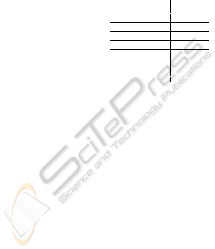
Table 1: Jeffers phonemes to viseme map (Jeffers and Bar-
ley, 1971). The last viseme, /S is used for silence. The table
shows the viseme visibility rank and occurrence rate in spo-
ken English.
Viseme
Visibility Occurrence TIMIT
Rank [%] Phonemes
/A 1 3.15 /f/ /v/
/B 2 15.49
/er/ /ow/ /r/ /q/ /w/
/uh/ /uw/ /axr/ /ux/
/C 3 5.88 /b/ /p/ /m/ /em/
/D 4 .70 /aw/
/E 5 2.90 /dh/ /th/
/F 6 1.20 /ch/ /jh/ /sh/ /zh/
/G 7 1.81 /oy/ /ao/
/H 8 4.36 /s/ /z/
/I 9 31.46
/aa/ /ae/ /ah/ /ay/ /eh/
/ey/ /ih/ /iy/ /y/
/ao/ /ax-h/ /ax/ /ix/
/J 10 21.10
/d/ /l/ /n/ /t/
/el/ /nx/ /en/ /dx/
/K 11 4.84 /g/ /k/ /ng/ /eng/
/S - - /sil/
maps, the viseme number is much higher, e.g. Gold-
schen map contains 35 visemes (Goldschen et al.,
1994).
In the first map, Jeffers & Barley group 43
phonemes into 11 visemes in the English lan-
guage (Jeffers and Barley, 1971) for what they de-
scribe “as usual viewing conditions”. The map link-
ing phonemes to visemes is shown in Table (1). In
this table visemes are labelled using a letter, from
/A to /K. To these 11, a silence viseme has been
added, labelled using /S. The last column is a sug-
gested phoneme to viseme mapping for the TIMIT
phoneme set. Two phonemes are not listed in the ta-
ble: /hh/ and /hv/. No specific viseme is linked to
them because, while the speaker is pronouncing /hh/
or /hv/, the lips are already in the position to produce
the following phoneme. Therefore /hh/ and /hv/ have
been merged with the following viseme. The table
shows the viseme visibility rank and occurrence rate
in spoken English (Jeffers and Barley, 1971). This
map is purely linguistic.
The second map analyzed is proposed by Neti et
al. (Neti et al., 2000). This map has been created us-
ing the IBM ViaVoice database and using a decision
tree, in the same fashion as decision trees are used
to identify triphones. Thus, this map can be con-
sidered a mixture of a linguistic and data driven ap-
proach. Neti’s map is composed by 43 phonemes and
12 classes (plus a silence class). Details are shown in
Table (2)
Hazen et al. (Hazen et al., 2004) use a data
driven approach. They perform bottom-up clustering
using models created from phonetically labelled vi-
sual frames. The map obtained is “roughly” (Hazen
et al., 2004) based on this clustering technique. The
PHONEME-TO-VISEME MAPPING FOR VISUAL SPEECH RECOGNITION
323

Table 2: Neti map (Neti et al., 2000).
Code Viseme Class Phonemes in Cluster
V1
/ao/ /ah/ /aa/
/er/ /oy/ /aw/ /hh/
V2 Lip-rounding /uw/ /uh/ /ow/
V3 based vowels /ae/ /eh/ /ey/ /ay/
V4 /ih/ /iy/ /ax/
A Alveolar-semivowels /l/ /el/ /r/ /y/
B Alveolar-fricatives /s/ /z/
C Alveolar /t/ /d/ /n/ /en/
D Palato-alveolar /sh/ /zh/ /ch/ /jh/
E Bilabial /p/ /b/ /m/
F Dental /th/ /dh/
G Labio-dental /f/ /v/
H Velar /ng/ /k/ /g/ /w/
S Silence /sil/ /sp/
Table 3: Hazen map (Hazen et al., 2004).
Viseme Class Phonemes Set
OV /ax/ /ih/ /iy/ /dx/
BV /ah/ /aa/
FV /ae/ /eh/ /ay/ /ey/ /hh/
RV /aw/ /uh/ /uw/ /ow/ /ao/ /w/ /oy/
L /el/ /l/
R /er/ /axr/ /r/
Y /y/
LB /b/ /p/
LCl /bcl/ /pcl/ /m/ /em/
AlCl /s/ /z/ /epi/ /tcl/ /dcl/ /n/ /en/
Pal /ch/ /jh/ /sh/ /zh/
SB /t/ /d/ /th/ /dh/ /g/ /k/
LFr /f/ /v/
VlCl /gcl/ /kcl/ /ng/
Sil /sil/
reason for this apparent inaccuracy is that the clus-
tering results vary a lot depending on the visual fea-
ture used. Hazen et al. group 52 phonemes into 14
visemes (plus a silence viseme). This is shown in Ta-
ble (3).
Bozkurt et al. (Bozkurt et al., 2007) created a map
using the linguistic approach. The map is based on
Ezzat and Poggio’s work (Ezzat and Poggio, 1998), in
which they define the phoneme clustering as “done in
a subjective manner, by comparing the viseme images
visually to assess their similarity”. The Bozkurt map
comprises 15 viseme (plus a silence viseme), and 45
phonemes detailed in Table (4).
In the final map shown in Table (5), Lee and
Yook (Lee and Yook, 2002) identify 13 (plus a si-
lence viseme) viseme classes from 39 phonemes (plus
a silence phoneme and a pause phoneme). They do
not explain how the map has been derived, so it has
Table 4: Bozkurt Map (Bozkurt et al., 2007).
Viseme Class Phonemes Set
S sil
V2 ay, ah
V3 ey, eh, ae
V4 er
V5 ix, iy, ih, ax, axr,y
V6 uw, uh, w
V7 ao, aa, oy, ow
V8 aw
V9 g, hh, k, ng
V10 r
V11 l, d, n, en, el, t
V12 s, z
V13 ch, sh, jh, zh
V14 th, dh
V15 f, v
V16 m, em, b, p
Table 5: Lee Map (Lee and Yook, 2002).
Viseme Class Phonemes Set
P b p m
T d t s z th dh
K g k n ng l y hh
CH jh ch sh zh
F f v
W r w
IY iy ih
EH eh ey ae
AA aa aw ay ah
AH ah
AO ao oy ow
UH uh uw
ER er
S sil
been assumed it is a linguistic map. Even though
they claim this is a many-to-one map, some phonemes
are mapped into 2 visemes, so the map is a many-to-
many map. To remove this ambiguity, in such cases
phonemes are associated with the first viseme pro-
posed. This affects 5 vowel phonemes.
It is not a simple task to compare these maps be-
cause the total viseme number and the total phoneme
number are different in the five maps. Table 6 sums
up the most relevant map properties. It is clear that
some similarities are present, particularly between the
Jeffers and Neti maps. In these two maps 5 con-
sonant classes are identical. Across all maps, the
consonant classes show similar class separation. All
the maps have a specific class for phoneme clusters
{/v/, /f/} and {/ch/, /jh/, /sh/, /zh/}. Jeffers, Neti,
ICPRAM 2012 - International Conference on Pattern Recognition Applications and Methods
324

Table 6: Map properties. Clustered phoneme number, num-
ber of visemes and number of vowel visemes. Silence
viseme and phonemes are not taken into consideration.
Map Phonemes
Total Vowel
Visemes Visemes
Jeffers 43 11 4
Neti 42 12 4
Hazen 52 14 5
Bozkurt 45 15 7
Lee 39 13 7
Bozkurt and Lee have a specific class for {/b/, /m/
/p/}. Group {/th/, /dh/} formsa viseme in Jeffers, Neti
and Bozkurt, while in Hazen and Lee it is mergedwith
other phonemes. Aside from this, the Hazen map (the
only data driven map) is significantly different from
the others, while Jeffers and Neti have an impressive
consonant class correspondence.
In contrast, vowel visemes are quite different from
map to map. The number of vowel visemes varies
from 4 to 7, and a single class can contain from 1
up to 10 vowels. No specific cross-map patterns are
present within maps.
A final difference within the maps is that the
phonemes {/pcl/, /tcl/, /kcl/, /bcl/, /dcl/, /gcl/, /epi/}
are not considered in the analysis by Jeffers, Neti,
Bozkurt and Lee, while they are spread across several
classes by Hazen.
3 FEATURE EXTRACTION
Feature extraction is performed in two consecutive
stages, a Region of Interest (or ROI) has to be detected
and then a feature extraction technique is applied to
the area. The ROI is found using a semi-automatic
technique (Cappelletta and Harte, 2010) based on two
stages: the speaker’s nostrils are tracked and then, us-
ing those positions, the mouth is detected. The first
stage succeeds on the 74% of the database sentences,
so the remaining 26% has been manually tracked to
allow experimentation on the full dataset. The sec-
ond stage has 100% success rate. Subsequently the
ROI is rotated according to the nostrils alignment. At
this stage the ROI is a rectangle, but its size might
vary in each frame. Thus, ROIs are either stretched or
squeezed until they have the same size. The final size
is the mode calculated using all ROIs size.
Having defined the region of interest, a feature ex-
traction algorithm is applied to the ROI. Three differ-
ent appearance-based techniques were used: Optical
Flow; PCA (principal component analysis); and DCT
(discrete cosine transform).
Optical flow is the distribution of apparent veloci-
ties of movement of brightness pattern in an image.
The code used in (Bouguet, 2002) implements the
Lucas-Kanade technique (Lucas and Kanade, 1981).
The output of this algorithm is a two dimensional
speed vector for each ROI point. A data reduction
stage, or downsampling, is required. The ROI is di-
vided in d
R
× d
C
blocks, and for each block the me-
dian of the horizontal and vertical speed is calculated.
In this way d
R
· d
C
2D speed vectors are obtained.
PCA (also known as eigenlips in AVSR applica-
tions (Bregler and Konig, 1994)) and DCT are similar
techniques. They both try to represent a video frame
using a set of coefficients obtained by the image pro-
jection over an orthogonal base. While the DCT base
is a priori defined, the PCA base depends on the data
used. The optimal number of coefficients N (the fea-
ture vector length) is a key parameter in the HMM cre-
ation and training. A vector too short would lead to
a low quality image reconstruction, too long a feature
vector would be difficult to model with a HMM. DCT
coefficients are extracted using the zigzag pattern and
the first coefficient is not used.
Along with these features, first and second deriva-
tives are used, defined as follows:
∆
k
[i] = F
k
[i+ 1] − F
k
[i− 1]
∆∆
k
[i] = ∆
k
[i+ 1] − ∆
k
[i− 1]
(1)
where i represents the frame number in the video, and
k ∈ [1..N] represents the kth generic feature F value.
Used with PCA and DCT coefficients, ∆ and ∆∆ repre-
sent speed and acceleration in feature evolution. Both
∆ and ∆∆ have been added to PCA and DCT features.
While optical flow already represents ROI elements
speed, only ∆ has been tested with it.
Optimal optical flow and PCA parameters have al-
ready been investigated and reported by the authors
for this particular dataset (Cappelletta and Harte,
2011). Results showed that an increment of PCA vec-
tor length does not improve the recognition rate figure
with an optimal value of N = 15. The best perfor-
mance is obtained using ∆ and ∆∆ coefficients, with-
out the original PCA data. Similarly, the best perfor-
mance with optical flow was achieved using original
features with ∆ coefficients. In this case performance
is not affected by different downsampling configura-
tions. Thus, the 2 × 4+ ∆ configuration will be used
for experiments reported in this paper.
4 EXPERIMENT
4.1 VIDTIMIT Dataset
The VIDTIMIT dataset (Sanderson, 2008) is com-
PHONEME-TO-VISEME MAPPING FOR VISUAL SPEECH RECOGNITION
325
prised of the video and corresponding audio record-
ings of 43 people (24 male and 19 female), reciting
10 short sentences each. The sentences were chosen
from the test section of the TIMIT corpus. The selec-
tion of sentences in VIDTIMIT has full viseme cov-
erage for all the maps used in this paper. The record-
ing was done in an office environment using a broad-
cast quality digital video camera at 25 fps. The video
of each person is stored as a numbered sequence of
JPEG images with a resolution of 512 x 384 pixels.
90% quality setting was used during the creation of
the JPEG images. For the results presented in this pa-
per, 410 videos have been used and they have been
split in a training group (297 sentences) and a test
group (113 sentences). The two groups are balanced
in gender and they have similar phoneme occurrence
rates. Training and test speakers did not overlap.
4.2 HMM Systems
HMMs were trained using PCA, DCT and optical flow
features. A visemic time transcription for VIDTIMIT
was generated using a forced alignment procedure
with monophone HMMs trained on the TIMIT au-
dio database. The system was implemented using
HTK. All visemes were modelled with a left-to-
right HMM, except silence which used a fully ergodic
model. The number of mixtures per state was grad-
ually increased, with Viterbi recognition performed
after each increase to monitor system performance.
No language model was used in order to assess raw
feature performance. The feature vector rate was in-
creased to 20ms using interpolation. Both a 3 and
4-state HMM were used.
The experiment was conducted in two stages. In
the first stage the Jeffers map was used. The HMM
and DCT feature parameters were varied in order to
find the optimal parameter configuration. It should
be noted that similar results were achieved using the
other maps but space limits the presentation of these
results to a single map. In particular, the recognition
rate is tested varying the HMM mixture number. Re-
sults are compared with PCA and optical flow feature
performance.
In the second stage of the experiments, the feature
set parameters were fixed (using the optimal configu-
rations in (Cappelletta and Harte, 2011) and those de-
termined for the DCT), in order to compare the results
from different maps. The optimal number of mixtures
for each individual viseme class was tracked. This
overcomes issues with different amounts of training
data in different classes. Thus HMMs used between 1
and 60 mixtures per state.
5 RESULTS
5.1 Feature Set Parameters
HMM results are assessed using the correctness esti-
mator, corr, defined as follows:
Corr =
T − D− S
T
× 100 (2)
where T is the total number of labels in the reference
transcriptions, D is the deletion error and S is the sub-
stitution error.
0 10 20 30 40 50 60
0
10
20
30
40
50
60
M − Mixture Number
Corr [%]
N14
N20
N27
N35
N44
N54
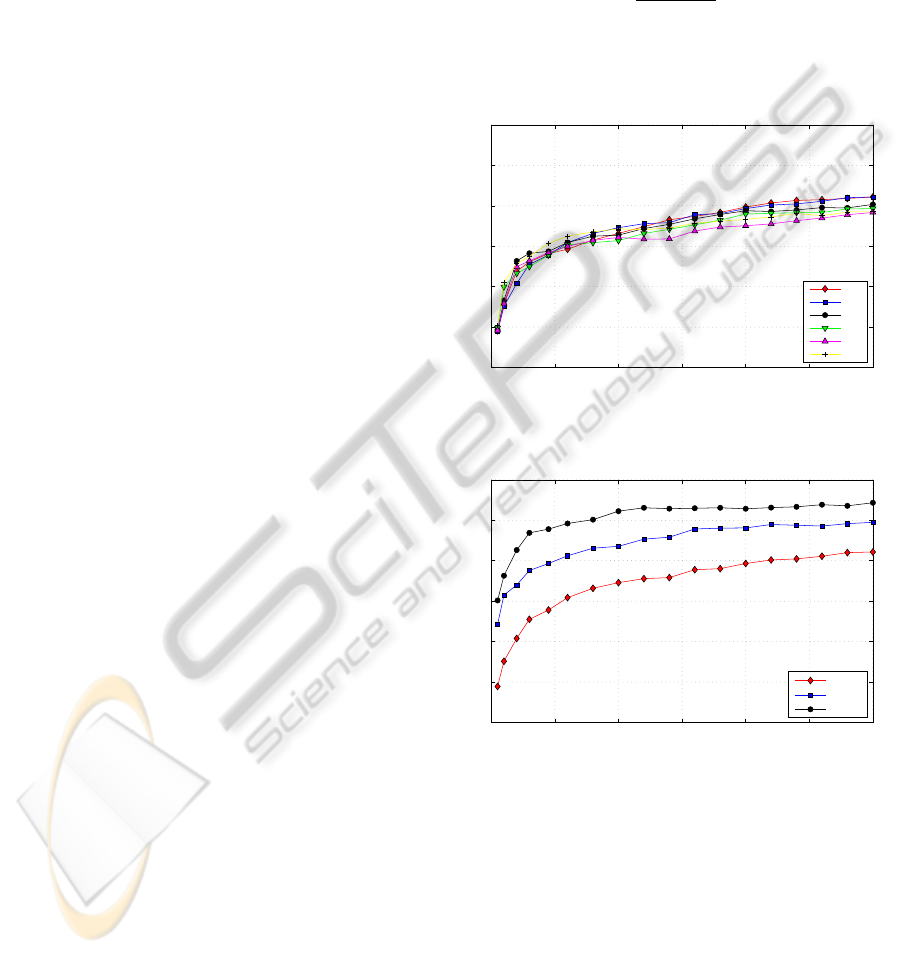
Figure 1: Basic DCT test, 3 States. N14, N20 refer to num-
ber of DCT features at 14, 20 etc..
0 10 20 30 40 50 60
0
10
20
30
40
50
60
M − Mixture Number
Corr [%]
DCT
DCT+∆
∆∆
Figure 2: Higher order DCT features. N = 20, 3 States. DCT
denotes 20 DCT features only, DCT+∆ denotes addition of
first order dynamics, ∆∆ denotes inclusions of both first and
second order dynamics without original DCT coefficients.
Figures 1 and 2 show the correctness of the 3-state
HMM using DCT features and the Jeffers map. Results
for the 4-state HMM are not shown because no sig-
nificant improvement from the 3-state was achieved.
Figure 1 shows the results of the basic DCT coefficient
tests obtained by varying the feature vector length N
between 14 and 54. The best results are achieved with
a vector length of 14 and 20, even though all the con-
figurations achieve very similar results, according to
ICPRAM 2012 - International Conference on Pattern Recognition Applications and Methods
326
Heckmann et al. (Heckmann et al., 2002). Signifi-
cant improvement can be achieved using ∆ and ∆∆.
Figure 2 shows the performance of 20 DCT coeffi-
cients with first and second derivatives added. The
recognition rate is increased by at least 30%. This be-
haviour mirrors that of the PCA feature set. As might
be expected, no significant improvement is achieved
behind 35 Gaussian mixtures.
5.2 Maps Comparison
In the second part of the experiment, all the maps
were tested. The PCA and DCT results are obtained
using ∆ and ∆∆ coefficients only, using N = 15 for
PCA, and N = 20 for the DCT feature set. Optical flow
results are obtained using 2×4 downsampling with ∆
coefficients. Along with correctness, defined in equa-
tion 2, it is advisable to use the accuracy estimator to
give a better overall indication of performance. The
standard definition was used:
Acc =
T − D− S− I
T
× 100 (3)
where I is the number of insertions.
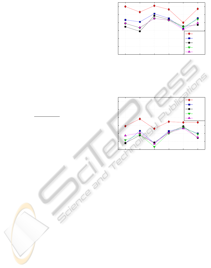
Figure 3 and Figure 4 show recognition results
for the five maps. When examining the figures, it is
important to realise that recognition results in a con-
tinuous speech task are expected to be relatively low
when compared to, for example, an isolated digit task.
It can certainly be argued that results will improve
significantly with use of a language model and when
combined with audio cues. However, this viseme set
exploration is seeking to study baseline viseme per-
formance initially.
It is apparent that the Jeffers map gives the best
results both in terms of correctness and accuracy. The
Neti map is the next best map, with little difference
in performance from the remaining maps. Examin-
ing the accuracy figures, it is clear that the insertion
level remains high overall. An insertion penalty was
investigated in an attempt to address this issue but a
suitable balance has not yet been found for the sys-
tem. The performance for the optical flow and PCA
features using 3-state HMMs was little better than a
guess rate.
It is possible to see a correlation between recogni-
tion rate and the number of viseme and vowel classes
listed in Table 6. The lower the viseme and vowel
class number, the better the recognition figure. Whilst
this is fully expected in a pattern recognition task, it is
still interesting to compare the Jeffers and Neti maps
because, even though many visemes encompass the
same phonemes (5 classes are identical), the results
are quite different. Results from 3-states HMM with
optical flow feature are used to demonstrate this, but
0
10
20
30
40
50
60
PCA−3
DCT−3
Optical Flow−3
PCA−4
DCT−4
Optical Flow−4
Corr [%]
Jeffers
Neti
Hazen
Bozkurt
Lee
Figure 3: 3- and 4-states HMM correctness for each map,
using all feature extraction techniques. Jeffers map gets
the best performance in all tests, considering both 3- and
4-states.
0
10
20
30
40
50
60
PCA−3
DCT−3
Optical Flow−3
PCA−4
DCT−4
Optical Flow−4
Acc [%]
Jeffers
Neti
Hazen
Bozkurt
Lee
Figure 4: 3- and 4-states HMM accuracy for each map, using
all feature extraction techniques. While Jeffers map still
gets good results, some maps reach the guessing rate level
(different for each map, see Table 6).
other feature sets yield similar conclusions. Figure 5
and Figure 6 show the confusion matrices obtained
using 3-states HMM optical flow tests. Total label
number, deletion number and substitution number are
also provided (see equation 2).
As expected the 5 identical classes (/H≡B, /F≡D,
/C≡E, /E≡F and /A≡G ) obtain basically the same
results. Thus, the Neti performance gap has to be
in the remaining consonant classes and in the vowel
visemes. Considering the vowel classes, it is possible
to see that in terms of number of phonemes covered,
Jeffers has two big (/B and /I) and two very small (/D
and /G) vowel classes. In contrast, Neti has four quite
balanced vowel classes (V1-V4 contain almost the
same number of phonemes). Jeffers has an advantage
because misclassification is less probable if classes
are big (see /B and /I in Figure 5). Moreover, even
a complete misclassification in the two small classes
will have a minor impact on the overall recognition
PHONEME-TO-VISEME MAPPING FOR VISUAL SPEECH RECOGNITION
327

Figure 5: Confusion matrix obtained with 3-states HMM us-
ing optical flow feature and Jeffers map. /B, /D, /G and /I
are the vowel visemes. Sub column represents the substitu-
tion error for each viseme, while del represents the deletion
error for each viseme. T = 3523, D = 420, S = 955 (see eq.
2).
rate. Figure 5 shows that /D and /G are basically com-
pletely misclassified, mostly in favour of the other two
vowel classes /B and /I, but these classes have such a
low occurrence that this misclassification is negligi-
ble from a statistical point of view. On the contrary,
Neti vowel visemes are more frequently misclassified.
They contribute roughly 60% more classification er-
ror, either in substitution or deletion errors.
Similar behaviour is present in the remaining con-
sonant classes. The remaining consonant phonemes
are clustered in two visemes in Jeffers map (/K and
/J) and in three visemes in Neti map (A, H and C).
Once again, the lesser the class number, the better the
classification. The three Neti visemes contribute 40%
more error than the two Jeffers consonant visemes.
6 CONCLUSIONS AND FUTURE
WORK
This paper has presented a continuous speech recog-
nition system based purely on HMM modelling of
visemes. A continuous recognition task is signifi-
cantly more challenging than isolated word recogni-
tion task such as digits. In terms of AVSR, it is a more
complete test of a system’s ability to capture pertinent
information from a visual stream, as the complete
set of visemes is present in a greater range of con-
texts. Five viseme maps have been tested, all based on
the phonemes-to-viseme map technique. These maps
were created using different approaches (linguistic,
data driven and mixed). A pure linguistic map (Jef-
Figure 6: Confusion matrix obtained with 3-states HMM us-
ing optical flow feature and Neti map. V1 to V4 are the
vowel visemes. Sub column represents the substitution er-
ror for each viseme, while del represents the deletion error
for each viseme. T = 3662, D = 531, S = 1262 (see eq. 2).
fers) achieved the best recognition rates in all the per-
formed tests. Compared with the second best map
(Neti), this improvement in performance can be at-
tributed to better clustering in some consonant classes
and less vowel visemes (statistically, Jeffers visemes
/D and /G are negligible).
Work is ongoing to extend this system to include
other feature sets including other optical flow im-
plementations and Active Appearance Model (AMM)
features to provide a definitive baseline for visual
speech recognition. To validate whether the Jeffers
map is a better approach to viseme modeling in the
context of a full AVSR system, the maps are also be-
ing tested incorporating speech features. This will test
the hypothesis that better visual features should im-
provethe overall AVSR performance when the speech
quality is low.
Unfortunately, the phonemes-to-viseme map ap-
proach does not take into account audio-visual asyn-
chrony (Potamianos et al., 2003; Hazen, 2006), nor
the fact that some phonemes do not require the use
of visual articulators, such /k/ and /g/ (Hilder et al.,
2010). Thus, along with the tested maps, it is impor-
tant to include in the analysis viseme definitions that
do not assume a formal link between acoustic and vi-
sual speech cues. This will emphasize the dynamics
in human mouth movements, rather than the audio-
visual link only.
To this end, the availability of large continuous
speech AVSR datasets (as opposed to isolated word
tasks or databases containing a small number of sen-
tences), continues to be a hurdle in AVSR develop-
ment.
ICPRAM 2012 - International Conference on Pattern Recognition Applications and Methods
328

ACKNOWLEDGEMENTS
This publication has emanated from research con-
ducted with the financial support of Science Founda-
tion Ireland under Grant Number 09/RFP/ECE2196.
REFERENCES
Bouguet (2002). Pyramidal Implementation of Lucas
Kanade Feature Tracker. Description of the algorithm.
Bozkurt, Eroglu, Q., Erzin, Erdem, and Ozkan (2007).
Comparison of phoneme and viseme based acoustic
units for speech driven realistic lip animation. In
3DTV Conference, 2007, pages 1–4.
Bregler and Konig (1994). ‘Eigenlips’ for robust speech
recognition. In Acoustics, Speech, and Signal Pro-
cessing, 1994. ICASSP-94., 1994 IEEE International
Conference on, volume ii, pages II/669–II/672 vol.2.
Cappelletta and Harte (2010). Nostril detection for robust
mouth tracking. In Irish Signals and Systems Confer-
ence, pages 239 – 244, Cork.
Cappelletta, L. and Harte, N. (2011). Viseme defini-
tios comparison for visual-only speech recognition.
In Proceedings of 19th European Signal Processing
Conference (EUSIPCO), pages 2109–2113.
Ezzat and Poggio (1998). Miketalk: a talking facial display
based on morphing visemes. In Computer Animation
98. Proceedings, pages 96–102.
Goldschen, A. J., Garcia, O. N., and Petajan, E. (1994).
Continuous optical automatic speech recognition by
lipreading. In Proceedings of the 28th Asilomar Con-
ference on Signals, Systems, and Computers, pages
572–577.
Hazen (2006). Visual model structures and synchrony con-
straints for audio-visual speech recognition. Audio,
Speech, and Language Processing, IEEE Transactions
on, 14(3):1082–1089.
Hazen, Saenko, La, and Glass (2004). A segment-based
audio-visual speech recognizer: data collection, de-
velopment, and initial experiments. In Proceedings of
the 6th international conference on Multimodal inter-
faces, pages 235–242, State College, PA, USA. ACM.
Heckmann, Kroschel, Savariaux, and Berthommier (2002).
DCT-Based Video Features for Audio-Visual Speech
Recognition. In International Conference on Spoken
Language Processing, volume 1, pages 1925–1928,
Denver, CO, USA.
Hilder, Theobald, and Harvey (2010). In pursuit of
visemes. In International Conference on Auditory-
visual Speech Processing.
Jeffers and Barley (1971). Speechreading (Lipreading).
Charles C Thomas Pub Ltd.
Lee and Yook (2002). Audio-to-Visual Conversion Using
Hidden Markov Models. In Proceedings of the 7th Pa-
cific Rim International Conference on Artificial Intel-
ligence: Trends in Artificial Intelligence, pages 563–
570. Springer-Verlag.
Lucas and Kanade (1981). An iterative image registration
technique with an application to stereo vision. In Pro-
ceedings of Imaging Understanding Workshop.
Neti, Potamianos, Luettin, Matthews, Glotin, Vergyri, Si-
son, Mashari, and Zhou (2000). Audio-visual speech
recognition. Technical report, Center for Language
and Speech Processing, The Johns Hopkins Univer-
sity, Baltimore.
Pandzic, I. S. and Forchheimer, R. (2003). MPEG-4 Facial
Animation: The Standard, Implementation and Appli-
cations. John Wiley & Sons, Inc., New York, NY,
USA.
Potamianos, Neti, Gravier, Garg, and Senior (2003). Recent
advances in the automatic recognition of audio-visual
speech. Proceeding of the IEEE, 91(9):1306–1326.
Saenko, K. (2004). Articulary Features for Robust Visual
Speech Recognition. Master thesis, Massachussetts
Institute of Technology.
Sanderson (2008). Biometric Person Recognition: Face,
Speech and Fusion. VDM-Verlag.
PHONEME-TO-VISEME MAPPING FOR VISUAL SPEECH RECOGNITION
329
