DETECTION OF LANE DEPARTURE ON HIGH-SPEED ROADS

David Hanwell and Majid Mirmehdi

University of Bristol, Bristol, U.K.

Keywords:

Lane departure, Lane tracking, Vanishing point.

Abstract:

We present a system for detecting and tracking the lanes of high-speed roads, in order to warn the driver of

accidental lane departures. The proposed method introduces a novel variant of the classic Hough transform,

better equipped to detect and locate linear road markings with a common vanishing point. This is combined

with a simple model of the lane and an Extended Kalman Filter to make detection and tracking more robust.

This allows detection of lane changes, resistant to visual interference by trafﬁc and irrelevant road markings.

1 INTRODUCTION

Studies have shown that many accidents are caused

by drivers falling asleep (Horne and Reyner, 1995),

especially during long journeys on high speed roads.

In such cases, mortality rates tend to be higher as

the driver is not sufﬁciently alert to brake or steer

to avoid obstacles (NCSDR/NHTSA Expert Panel on

Driver Fatigue and Sleepiness, 1998). Even when

wide awake, a driver’s inattentiveness can cause ac-

cidents, e.g. due to failure to check for other vehicles

in blind spots when changing lanes. Recently, some

vehicle manufacturershavebegun to incorporate cam-

eras into their cars, for example to provide a more fa-

vorable rear-view when reversing. Using these to pro-

duce a lane departure warning system (LDWS) could

help reduce both the number and severity of accidents

(Rimini-Doering et al., 2005).

For its use to become widespread, a LDWS should

be as cheap and simple to install as possible, requiring

minimal additional hardware. Much of the previous

work in lane detection and tracking looks at the more

involved problem of autonomous driving, requiring

extra hardware for a more elaborate approach to lane

departure detection, e.g. many use multiple cameras

(Loose and Franke, 2010; Lipski et al., 2008).

Accidental lane departures are most common, and

most dangerous,on high speed roads. Such roads tend

to have low curvature, appearing almost straight, es-

pecially from our camera’s viewpoint, mounted on the

front bumper signiﬁcantly below driver eye view (see

Fig. 5(a) for an example). We exploit this fact to sim-

plify both the detection and modelling of lane mark-

ings and present a system which uses only a single

camera, and requires no more computational power

than provided by a standard PC. The data is obtained

from an experimental vehicle by Jaguar Land Rover.

In order for a LDWS to be effective, it must be

resilient to visual clutter. Speciﬁcally, it should (a)

detect only those image features which correspond to

road markings, i.e. ignore road barriers, or other traf-

ﬁc, (b) ignore irrelevant road markings, i.e. writing

on road surfaces or road markings not parallel to the

vehicle’s lane, and (c) be able to detect and track not

only those markings delimiting the vehicle’s immedi-

ate lane, but also adjacent lanes to allow tracking to

be uninterrupted during, and after, a lane change.

For each of the above criteria, one can ﬁnd exam-

ples of its use in previous work, but no single piece of

work incorporates all three into a single camera sys-

tem. In the case of the 1

for example, (Wu et al.,

2009) describes a system which exploited the con-

trast of road markings against their background. They

used transitions in image intensity, with a statistical

search algorithm, to ﬁnd road markings. Most others

however, simply sought strong edge lines (McDon-

ald, 2001; Voisin et al., 2005; Jung and Kelber, 2005).

While road markings do tend to have strong edges, not

all strong edges correspond to road markings, and so

it can be prone to interference, e.g. from other trafﬁc.

Approaches to the 2

criteria usually involve tak-

ing into account the expected position and orienta-

tion of road markings. For example in (McDonald,

2001), the vanishing point (VP) of the road markings

was presumed to lie in a ﬁxed rectangular region of

the image. A Hough transform (HT) was applied to

this rectangle, and the accumulator binarised, giving

a map of the points in the Hough space that represent

lines which pass through the rectangular region. This

was then used as a mask for the accumulator during

529

Hanwell D. and Mirmehdi M. (2012).

DETECTION OF LANE DEPARTURE ON HIGH-SPEED ROADS.

In Proceedings of the 1st International Conference on Pattern Recognition Applications and Methods, pages 529-536

DOI: 10.5220/0003732605290536

 SciTePress

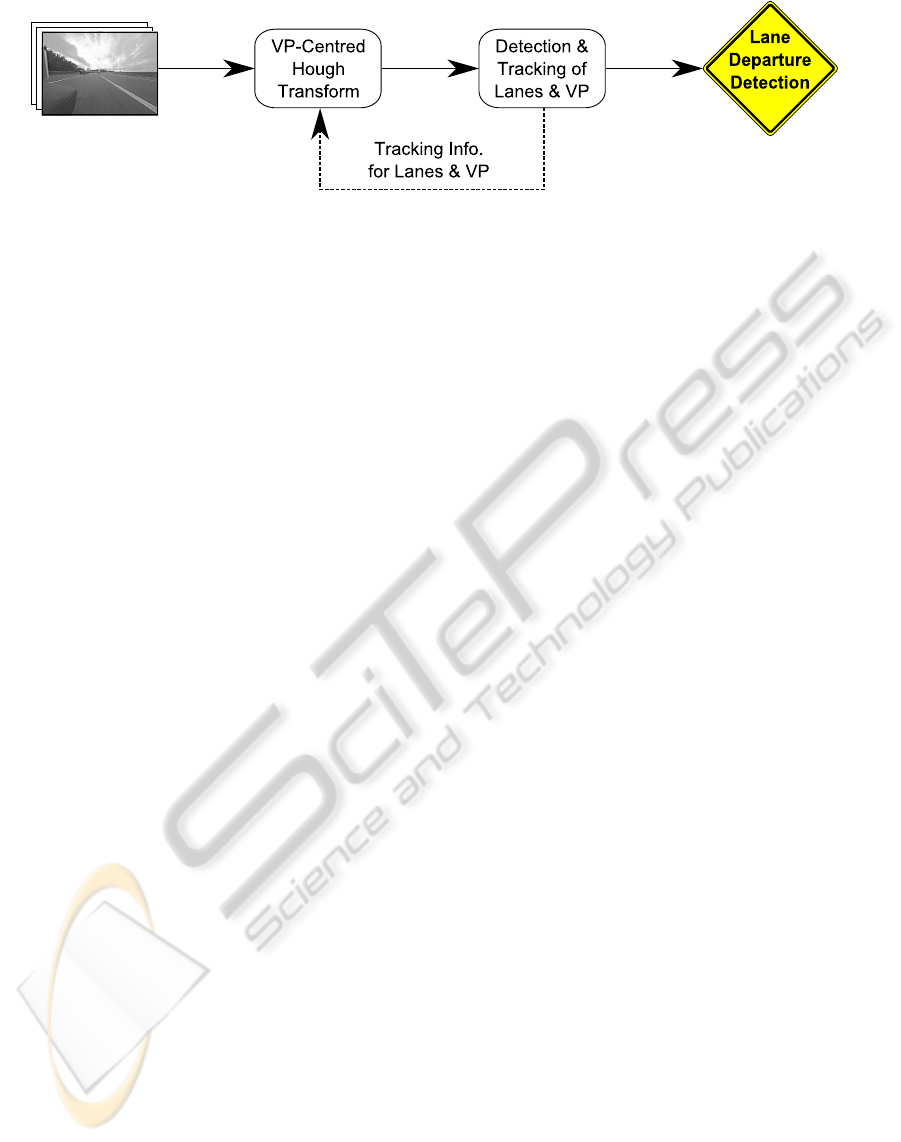
Figure 1: An overview of the system.

the detection of lane edge lines, thus ﬁltering out any

detected edges unlikely to belong to road lane mark-

ings. In (Jung and Kelber, 2005), a histogram of edge

pixel directions was used in a weighted HT to extract

the edge lines in the most common directions. The

authors state this worked well but could be prone to

interference from other ‘signiﬁcant structures’ in the

image, or from vehicles close in front.

Of the three criteria, the 3

is perhaps the least

common, with most previous work concentrating on

tracking only two (Voisin et al., 2005; Wu et al., 2009;

Jung and Kelber, 2005) or three (McDonald, 2001;

D’Cruz and Jia Zou, 2007) road markings. One no-

table exception is (Ieng et al., 2005), in which arbitrar-

ily many road markings were simultaneously tracked,

each with a separate Kalman ﬁlter (KF). However, the

width of each lane was not taken into account, and

multiple cameras were required.

While many of the above showgood results in lane

tracking, none take into account all three criteria, and

so are not ideally suited to LDWS. We propose a sim-

ple LDWS method that detects and tracks the lanes

of high speed roads, and addresses all three crite-

ria. We demonstrate insensitivity to both nearby traf-

ﬁc and irrelevant road markings. Our method begins

with a novel variant of the classic HT which is bet-

ter equipped to detect and locate linear road markings

with a common VP (Section 4). It uses knowledge

of the VP location to detect only those road markings

parallel to the lane. Also, it takes advantage of the

distinctive appearance of linear road markings, to dis-

tinguish them from other lines parallel to the lane, e.g.

edges of vehicles or road barriers. This is combined

with an Extended Kalman Filter (EKF) to detect (Sec-

tion 4.1) and track (Section 4.2) arbitrarily many road

markings which are then used to estimate the VP lo-

cation by an MSE minimisation method (Section 5).

The VP is tracked between frames using a KF, and

used by the HT to allow it to ignore edge lines not

parallel to the lane. Its y-coordinate is used to deﬁne

the ROI, allowing us to ignore objects above the hori-

zon. A system overview is shown in Fig. 1. Section 6

presents our results, and demonstrates the robustness

of our system on both straight and curved sections

of high-speed roads, and its robustness to occlusions.

The paper is concluded in Section 7.

2 CAMERA-VEHICLE SET-UP

Footage was taken using a colour video camera

mounted on the front bumper of the vehicle, 58cm

above the ground. The camera has a horizontal ﬁeld

of view of 157°, resulting in severe ﬁsh-eye distor-

tion, making a correction necessary. The result is an

anti-aliased, greyscale image, conforming to a recti-

linear projection. Mounted so low, the camera gives a

different view from that usually seen by a driver (see

Fig. 5(a)). It points forward, so that the horizon is ap-

proximately halfway up the image, allowing us to ig-

nore the upper part of the image once the VP is found.

Also, because the camera is mounted so low down,

more distant road is contained within a much smaller

area of image than nearer road, making more distant

road markings difﬁcult to distinguish. However, the

low camera position causes road markings in the im-

age to be less affected by the road’s curvature, allow-

ing the system to function well even on curves. The

choice of lens and camera position was not ours, but

that of the vehicle manufacturer. The camera is one

of six ﬁtted to this model of vehicle, serving a variety

of purposes including reversing and parking aids.

3 THE ROAD MARKING MODEL

In order to determine whether the vehicle has crossed

a lane boundary, we must model the relationship be-

tween lines in the ground plane, and their correspond-

ing lines in the image. This relationship is used to

facilitate the detection and tracking of road markings.

We use a standard pinhole camera model, with viewer

axes X, Y, and Z, whose origin is the focal point. Our

image plane has axes x and y, which lie parallel to the

X and Y axes respectively.

We deﬁne a coordinate system in the ground

plane, with axes u and v, and origin at (0,h,0) in

ICPRAM 2012 - International Conference on Pattern Recognition Applications and Methods

530

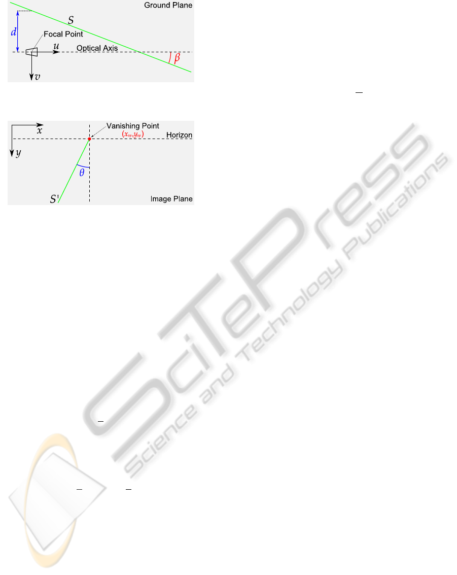
Figure 2: A top-down view of the parametrization of lines

in the ground plane.

Figure 3: The parametrisation of lines in the image plane,

relative to the VP.

the viewer coordinate system, where h is the camera

height above the ground. The v axis is parallel to the

X and x axes, but the u axis is not necessarily parallel

to the Z axis, due to the tilt, α, of the camera relative

to the ground plane.

Now consider a straight line, S in the ground

plane, such as a road marking’s edge line, and assume

that the VP of S in the image has already been de-

termined to be at (x

) (Section 5). The line S is

parametrised by (d,β), where d is its distance from

the uv-axes origin along the v axis, and β is the angle

at which it meets the u axis (Fig. 2). Hence, it is de-

ﬁned by v = utanβ− d. The corresponding line in the

image plane, S

′

(Fig. 3) is then:

y− y

(x− x

). (1)

The line has slope h/d, hence a line in the ground

plane parametrised by (d,β) will lie in the image

plane at θ, i.e.

θ =

+ tan

−1





. (2)

Thus, the lateral position, d, of a detected edge line in

the ground plane relative to the camera, depends only

upon θ, the angle at which it was detected, and so is

invariant to translation. Crucially, this means that as

long as we know the road markings’ collective VP,

we can describe the location of each using only one

value, θ. This has two implications: ﬁrstly, it means

we can separate the tracking of the VP and the road

markings into two independent tasks, and secondly,

it means that to track a road marking, we need only

store its angle between frames.

In determining a white lane marking, we are in-

terested in ﬁnding the pair of edge lines demarcat-

ing it. Suppose θ

and θ

are the angles of two edge

lines in the image. We wish to determine the relation-

ship between these two angles, and the perpendicu-

lar distance w, between the corresponding lines in the

ground plane. Using (2) we can derive,

= g(θ

,w) = tan

−1



− tan(−θ

)



. (3)

Hence, if we detect two road markings, we can deter-

mine the distance between them, and having detected

one edge line of a road marking we can estimate the

range of angles in which the other will lie.

4 NOVEL VARIANT OF THE HT

We begin by applying both horizontal and vertical

Scharr ﬁlters (J¨ahne et al., 1999) to the greyscale in-

put frame, to produce two gradient maps. Only those

pixels whose gradient magnitude is above a (liber-

ally selected) threshold go on to be represented in

the Hough accumulator. When transforming an edge-

pixel to the accumulator, instead of making an entry

for every value of θ, we instead use only a narrow

range, 2° each side of the edge-pixel’s angle. This is

intended to increase the speed at which the HT can

be performed, and to increase accuracy by reducing

the likelihood of erroneous maxima in the accumu-

lator. An edge pixel’s additions to the accumulator

are weighted in proportion to its gradient. This re-

sults in shorter, more well deﬁned edge lines being

favoured over longer, more weakly deﬁned ones. A

similar modiﬁcation was made in (Jung and Kelber,

2005) for the same reason.

Parallel road markings have a common VP in

the image. We distinguish between those edge lines

which pass through or close to this VP, and those

which do not by ﬁrst estimating the location of the VP,

and then performing a translation of image coordi-

nates, moving the origin to this estimated VP. We are

then able to exploit the polar coordinate system inher-

ent to the HT, by restricting the distance dimension, ρ,

of the accumulator to a narrower range, and thus omit

the parametrisations of lines which pass too far from

the VP. This amounts to only considering lines which

pass through a small circular region centred at the VP

(Fig. 4). By tracking the VP, we allow this efﬁciency

to continue for subsequent frames. This detection and

tracking is expounded on in Section 5.

This contrasts with the method of (McDonald,

2001) in which the VP is not explicitly detected, but

presumed to lie in a ﬁxed rectangular region of the

image. A mask for the Hough accumulator speciﬁes

DETECTION OF LANE DEPARTURE ON HIGH-SPEED ROADS

531

which parametrisations correspond to lines that pass

through this rectangle. A possible shortcoming of this

approach is that should the VP move out of the rect-

angle, none of the lane markings would be detected.

In order to move or resize the detection region, a new

mask would have to be created. Our method allows

the image region through which lane edge lines must

pass to be moved and resized as necessary, with no

increase in computation, with its radius, φ, based on

the covariance matrix of the VP KF (see Fig. 4). Fur-

thermore, our method uses a smaller accumulator in

which maxima can be found more quickly.

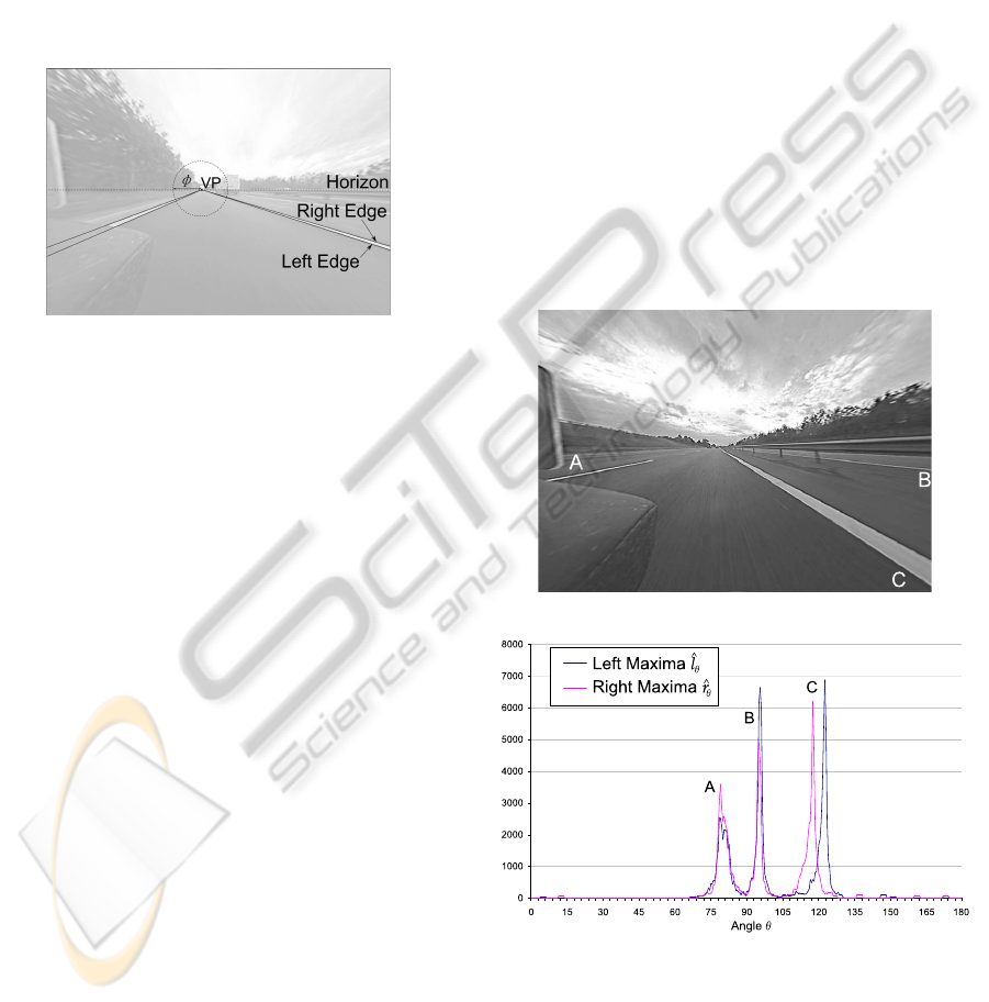
Figure 4: The circle of detection, and left and right edges.

Road markings are, by design, among the bright-

est objects on the road and have deﬁnite edges along

the transition from bright white paint to darker grey

road material. Since they are of constant width, they

have two parallel edge lines of opposite gradient di-

rection. We exploit both the sharpness of these gra-

dients, and the fact that they occur in converse pairs,

to distinguish them from other objects parallel to the

lane, such as barriers and nearby vehicles.

Our accumulator is a 2D array, A(ρ, θ), where ρ

speciﬁes the perpendicular distance from a line to the

origin, and θ is the angle of the line. We refer to edge

pixels at which the image intensity increases in the

anti-clockwise direction about the VP, as the left edge

line of a road marking, and similarly, edge points at

which the image intensity increases in the clockwise

direction, as right edge line (Fig. 4). Each element of

the 2D accumulator stores two values, l and r, cor-

responding to left and right edges respectively, i.e.

A(ρ,θ) = (l,r).

Hence, the accumulator has two channels, a left

channel and a right channel. When performing the

HT, a pixel’s gradient direction is used to determine

which edge type it lies upon, and its addition to the

accumulator is then made to the corresponding chan-

nel. This means each occurrence of a lane marking

is characterised in the accumulator by a pair of rel-

atively high values, not more than a certain distance

apart, with one being in each channel.

To facilitate the identiﬁcation of pairs of maxima

in the accumulator, the largest value is taken from

each column of each channel of the accumulator and

recorded along with the value of ρ at which it oc-

curred, i.e. we obtain for each of the (l,r) channels in

A, a 1D array of values, resulting in two arrays, L(θ)

and R(θ), which we refer to as the left maximum array

and the right maximum array respectively,

L(θ) = (

), R(θ) = (

, ˆr

) (4)

with,

= argmax



(ρ,θ)



(5)

= max



(ρ,θ)



(6)

where A

and A

are the left and right channels of

A respectively, and

and ˆr

are deﬁned similarly.

An example of a typical frame and a graph showing

the contents of the maximum arrays resulting from

our HT are shown in Fig. 5. The graph clearly shows

three pairs of peaks, each representing one of the three

road markings visible in the frame.

(a) A typical frame.

(b) A plot of the two maximum arrays derived from the Hough accumulator

for the frame above.

Figure 5: Labels A, B, C mark the correspondence of the

peaks in maxima arrays

and ˆr

to lane markings.

This reduction in dimension greatly simpliﬁes

lane marking detection, as we later describe. It makes

ICPRAM 2012 - International Conference on Pattern Recognition Applications and Methods

532

the assumption however, that for each θ-value, there

will be at most one relevant maximum in each accu-

mulator channel. This is equivalent to the assumption

that no two relevant edge lines will be parallel in the

image. We consider this to be a credible assumption

for two reasons. Firstly, most linear objects in the

road environment are parallel to the road, and hence

share the same VP in the image as the road lane. This

implies that their edge lines are not parallel in the im-

age. Secondly, to be detected, edge lines must pass

through a relatively small circle around the VP. If a

detected edge line does have a parallel elsewhere in

the image, it is unlikely that it will be detected.

To summarise, there are four key differences be-

tween our method and the classical HT method: (a)

edge direction is taken into account when applying

the transform to a pixel, (b) the values added to the

accumulator are proportional to gradient magnitudes,

mulator maxima corresponding to relevant edges lie

near ρ = 0, and (d) we use two accumulator channels

for left and right edges.

4.1 Road Marking Detection

Once the maximum arrays for a frame have been com-

puted, the average value is calculated over both ar-

rays. This givesa measure of the overall edge strength

in the frame, and is used to automatically set appropri-

ate thresholds for road marking detection. This is in-

tended to allow the system to quickly adapt to chang-

ing weather and light levels.

To simplify the process of detecting pairs of sig-

niﬁcant local maxima in the two maximum arrays, we

‘thin’ each array by suppressing secondary maxima.

For each value of θ, we imagine a line at that angle.

We use (3) to calculate what range of angles is likely

to represent lines in the ground plane which lie within

a small lateral distance w of that line. In the maximum

arrays, we keep only the largest value in the range,

and set the rest to zero. More formally, we replace

each

by f

(θ), where,

(θ) =







= max

′

∈G(θ,w)

′

0 otherwise

(7)

where G(θ, w) = [g(θ,−w),g(θ,w)] with g(θ,w) as

in (3). Values of ˆr

are treated similarly. The result is

a sparse set of peaks, corresponding to lines that meet

at the VP and we expect to be lane markings; for an

example see Fig. 6.

As shown in Section 3, we can deﬁne each line

parallel to the lane, by a single value, θ. We de-

scribe each road marking by the angle of its central

Figure 6: The data shown in Fig. 5(b) after ’thinning’.

line, by averaging the angles of its two edge lines.

Given this angle, and a maximal thickness of a linear

road marking w, we use (3) to determine the appropri-

ate range of θ to search in the maximum arrays. We

determine w empirically to be approximately 32cm.

To increase performance, the ranges of θ values are

calculated off-line and stored in an array. We require

peaks to be larger than a certain threshold, which is

proportional to the automatic edge strength measure

described above. We also impose other criteria, such

as a maximal ratio between the peaks’ values, and a

maximal difference between their corresponding ρ-

values. Once a road marking is detected, its central

angle is used to track it in the next frame.

Due to the lens and camera position employed in

our system, road markings close to the vehicle take

up a large proportion of the frame, and appear almost

straight even on curved roads. For this reason, our

method is appropriate even for roads of some curva-

ture, and is especially useful for a LDWS since nearer

road markings give the best indication of the vehicle’s

current position relative to the lane.

4.2 Tracking of Road Markings

To track road markings, we use an EKF (see the

model used in Fig. 7) which is able to track either

one or two road markings. The approach used is to di-

rectly track those road markings which are of immedi-

ate concern, i.e. the ones which delimit the vehicle’s

current lane. Then, the motion of the tracked mark-

ings is used to predict the locations of the road mark-

ings which are not tracked based on the assumption

that all relevant road markings are parallel, and thus

share the same lateral velocity relative to the camera.

This is particularly useful in maintaining the tracking

of dashed or occluded road markings

From (2) we can determine the position of a road

marking in the ground plane to be,

λ = tan(−θ), (8)

DETECTION OF LANE DEPARTURE ON HIGH-SPEED ROADS

533

where θ is the angle of the line in the image plane,

and λ is the lateral offset from the camera in units of

h. There are three quantities which comprise the ob-

servation of the lane. The ﬁrst two are the angles in

the image plane at which each of the left and right

lane boundary markings were detected, θ

and θ

re-

spectively. The third is the lateral velocity, ν, which

is measured using the changes in road markings’ po-

sitions between frames. We calculate their lateral po-

sition on the ground plane, determine the movement

of each, and take the mean. Lane width ψ is calcu-

lated as the difference in the lateral positions of the

two road markings delimiting the lane.

If one of the two lane boundary markings is not

detected in a frame, its position is inferred using the

position of the other, and the model’s current estimate

of the lane width, ψ. Should neither lane boundary

marking be detected, the model’s prediction is used as

the next model state, and the model state’s covariance

updated accordingly, bypassing the weighting and up-

date stages. This continues until either one or both

of the lane delimiting markings is explicitly detected,

or until one of them has been absent for a sufﬁcient

number of frames that it is deemed no longer to ex-

ist. Similarly, if no estimate of ν can be made, it is

assumed to remain constant.

4.3 Management of Road Markings

For each tracked road marking, we store details such

as its age (number of frames since ﬁrst detection) and

its recent absences (number of frames since last de-

tected), which are used to decide whether or not it

is a lane boundary. This increases robustness against

mis-detections, e.g. by requiring that a road marking

be detected in 4 consecutive frames before it is con-

sidered real. It also allows dashed and occluded road

markings to be maintained in the list despite not being

detected for severalframes at a time, while at the same

time not allowing such transient features as writing on

the road surface to be mistaken for lane delimiters.

• The distance from the camera

to the left of the lane, λ.

• The width of the lane, ψ.

• The lateral velocity of the

lane, relative to the camera, ν.

Figure 7: The model used in the EKF.

Given (8), we can calculate the lateral distance of

a road marking from the camera using its angle in the

image. We can hence determine whether the vehicle

is on top of, or close to, each road marking. This

allows us to deduce whether the driver is in danger

of making an accidental lane departure. We require

that the vehicle be within 15cm of a lane boundary, or

within 30cm and moving towards it, in order to trigger

an alarm. These limits are easily adjustable to suit.

Should the vehicle approach a lane boundary

quickly, this warning will occur very soon before the

vehicle actually crosses the boundary. In order to

warn the driver earlier, we use a third criterion which

combines the distance from the lane boundary with

the lateral velocity of the vehicle relative to it. In

(Godthelp et al., 1984) the distance of a lane bound-

ary from the vehicle is divided by the lateral veloc-

ity, to give a time-to-lane-crossing (TLC) value. We

use the same method, and trigger an alarm whenever

this TLC value falls below 25 frames. If employed

on an actual vehicle, this alarm could be suppressed

when the corresponding direction indicator is acti-

vated, thus detecting only accidental lane departures.

5 LOCATING & TRACKING THE

In (Cantoni et al., 2001) a method of estimating the

VP in an image was proposed that involved a MSE

minimization method to the contents of the Hough ac-

cumulator. We apply the same process but only to the

parameters of detected road markings. This means

fewer points must be processed, and, should the im-

age contain multiple VPs, we can be more certain that

we have identiﬁed the correct one.

Given N lines, parametrised by (ρ

,θ

) for i =

1,...,N, we estimate their VP ˆx

, ˆy

as:

ˆx

AE − CD

AB− C

, ˆy

BD− CE

AB− C

, (9)

where,

A =

∑

i=1

sin

, B =

∑

i=1

cos

, C =

∑

i=1

cosθ

sinθ

D =

∑

i=1

sinθ

, and E =

∑

i=1

cosθ

In order for a road marking’s position to contribute

to the estimate of VP location in a frame, it must have

been detected in that frame and be old enough to be

considered a genuine road marking (see Section 4.3).

Lookup tables are used to increase performance.

To track the VP, a simple KF is used, with a con-

stant position model consisting only of the VP’s co-

ordinates in the image. Though this is an almost triv-

ial instance of a KF, it has an important advantage

ICPRAM 2012 - International Conference on Pattern Recognition Applications and Methods

534

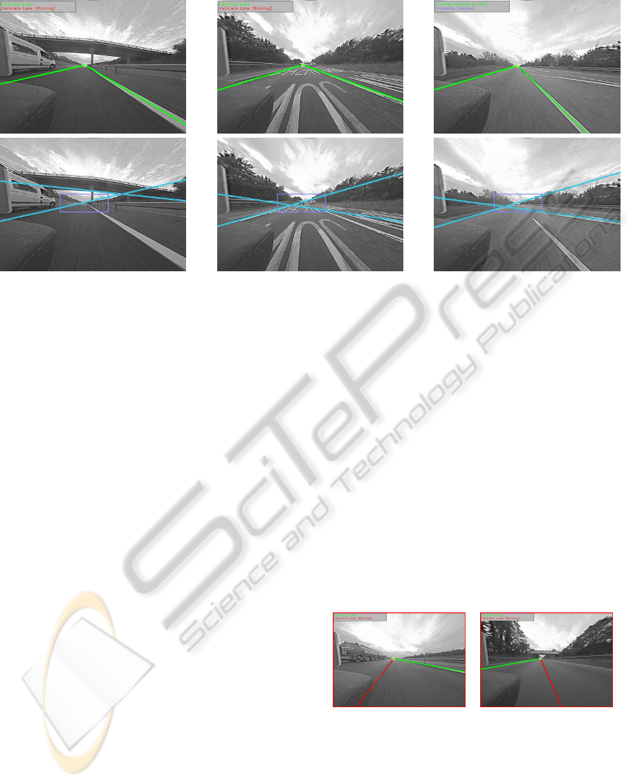
Figure 8: Our system (top) tracking lanes in the face of clutter, compared to McDonald (bottom).

over simpler methods such as exponential averaging.

There may be frames in which insufﬁcient road mark-

ings are found to give a reliable estimate of VP loca-

tion. In such cases we simply use the model’s predic-

tion of VP location (i.e. that it remains where it is),

but increase the model’s covariance. When the VP’s

location can again be observed, the model will have

higher variance, and so more weight will be given to

the observation, resulting in the VP returning more

quickly to its true coordinates. Quantitative experi-

ments conﬁrm that VP tracking accuracy is much im-

proved by the KF (Section 6).

As the location of the VP is used in the detection

of road markings, and the locations of road markings

are used to determine the VP, the system requires an

initial bootstrapping phase. This is achieved by ini-

tially setting the VP to be in the centre of the frame

and using a large radius of detection in the HT. As

road markings are detected, the covariance of the VP

KF decreases, and the radius of detection with it. In

our experiments, the VP KF typically takes around 1s

to converge to the correct location.

6 RESULTS

We present our results, comparing against those of

(McDonald, 2001), which is the closest work to

ours in methodology. Though there are currently

several commercially available LDWSs, we are un-

able to provide comparison with them as details of

their methodology remain undisclosed. These in-

clude Mobileye’s lane departure warning application

(Mobileye

N.V., 2010), which is integrated into sev-

eral manufacturers’ vehicles.

We also show examples of lanes being tracked de-

spite transient occlusions. In our approach, we esti-

mate the VP and do not process pixels above the hori-

zon. McDonald’s method does not locate the hori-

zon or VP, so in order to make the comparison fair

when applying McDonald’s method to our data, we

measured the ratio of image area above and below the

horizon in the examples shown in (McDonald, 2001),

and removed a portion of the frame in our data, to

achieve a similar ratio. In the examples, for McDon-

ald’s method, the rectangle through which lines must

pass in order to be detected is shown in lilac.

Fig. 9 shows two examples of lane change detec-

tion by the proposed method - in the left ﬁgure the ve-

hicle is crossing to the left and in the right it is about

to cross the lane to its right. Road markings being

crossed are shown in red.

Figure 9: Examples of lane changes being detected.

Fig. 8 demonstrates key advantages of the pro-

posed method. Firstly, strong edges not belonging to

road markings are not detected. McDonald’s method

(McDonald, 2001) is confused by strong edges, e.g.

in the 1

column of Fig. 8, the edge between the un-

derside of a bridge and the sky, is detected as a road

marking. Because (McDonald, 2001) only tracks two

DETECTION OF LANE DEPARTURE ON HIGH-SPEED ROADS

535

road markings, when some other object is mistaken

for a road marking, a real road marking goes unde-

tected. Our proposed method does not detect strong

non-lane edges for two reasons. Firstly, estimating

the VP allows everything above the horizon to be ig-

nored, and so other vehicles or objects on the roadside

have much less inﬂuence. Secondly, instead of sim-

ply detecting edge lines, our method requires them to

be correctly paired, and so edges which do not corre-

spond to road markings are not detected.

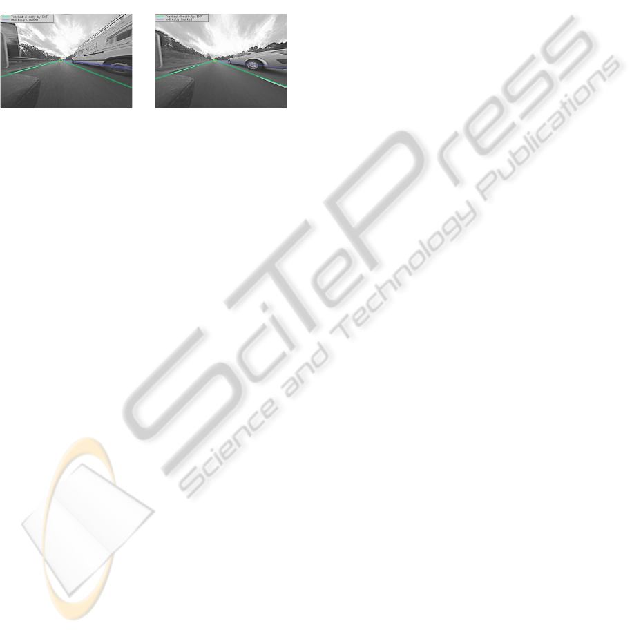
Figure 10: Lane markings being tracked through occlusion.

In general, our method shows high detection ac-

curacy and good resistance to visual clutter. As Fig.

8 demonstrates, McDonald’s method copes less well

with such interference. In these respects, we fulﬁl the

ﬁrst two of the criteria outlined in Section 1. Since we

track multiple road markings, our method also satis-

ﬁes the third criteria. Fig. 10 shows tracking of lane

markings through occlusion by nearby vehicles.

We performed a quantitativeassessment of our VP

tracking by ﬁrst manually determining the VP in 200

consecutive frames. Then we measured the distance

between the proposed method’s VP location and the

ground truth to have a mean of 2.0 pixels with a vari-

ance of 2.7. With the KF turned off, the mean was 4.4

pixels with a variance of 15.7.

Using a single thread on an Intel Core i5-660 CPU

at 3.33 GHz, our system can achieve an average per-

formance of 64 fps. The proposed method involves a

few parameters, for example, how long a road mark-

ing is tracked for before it is considered to be a lane

boundary, and how long one goes undetected before

it is dropped by the system. The values for all our

parameters have been empirically determined and re-

mained constant in all the experiments.

7 CONCLUSIONS

We described a novel variant of the HT for the detec-

tion and tracking of linear road markings, with several

novel reﬁnements to the classical HT method, includ-

ing the use of two accumulators and the translation of

image coordinates to put their origin at the VP to fa-

cilitate more efﬁcient analysis, such as ignoring road

markings which are not parallel to the lane. The VP

is also detected and tracked, and feeds back into the

HT process for subsequent frames. The method ex-

hibits real-time performance with spare capacity for

additional tasks.

ACKNOWLEDGEMENTS

The authors would like to thank Jaguar Land Rover

for their support and supply of videos.

REFERENCES

Cantoni, V., Lombardi, L., Porta, M., and Sicard, N. (2001).

Vanishing point detection: Representation analysis and

new approaches. In Proc. of ICIAP.

D’Cruz, C. and Jia Zou, J. (2007). Lane detection for driver

assistance and intelligent vehicle applications. In ISCIT

2007, pp. 1291–1296.

Godthelp, H., Milgram, P., and Blaauw, G. (1984). The de-

velopment of a time-related measure to describe driving

strategy. Human Factors: Journal of HFES.

Horne, J. A. and Reyner, L. A. (1995). Sleep related vehicle

accidents. BMJ, 310(6979):565–567.

Ieng, S.-S., Vrignon, J., Gruyer, D., and Aubert, D. (2005).

A new multi-lanes detection using multi-camera for ro-

bust vehicle location. In Proc. IEEE IV, pp. 700–705.

J¨ahne, B., Scharr, H., and K¨orkel, S. (1999). Handbook of

Computer Vision and Applications., pp. 125–152.

Jung, C. R. and Kelber, C. R. (2005). Lane following and

lane departure using a linear-parabolic model. Image and

Vision Computing, 23(13):1192–1202.

Lipski, C., Scholz, B., Berger, K., Linz, C., Stich, T., and

Magnor, M. (2008). A fast & robust approach to lane

marking detection & lane tracking. In SSIAI, pp. 57–60.

Loose, H. and Franke, U. (2010). B-spline-based road

model for 3d lane recognition. In Proc 13th Intelligent

Transportation Systems, pp. 91–98.

McDonald, J. (2001). Application of the HT to lane detec-

tion & following on high speed roads. In ISSC.

Mobileye

N.V. (2010). Lane Departure Warning.

http://www.mobileye.com.

NCSDR/NHTSA Expert Panel on Driver Fatigue and

Sleepiness (1998). Drowsy driving and automobile

crashes, Report No. DOT HS 808 707.

Rimini-Doering, M., Altmueller, T., Ladstaetter, U., and

Rossmeier, M. (2005). Effects of lane departure warning

on drowsy drivers performance and state in a simulator.

In 3rd Int. Driving Symp. on Human Factors in Driver

Assessment, Training, & Vehicle Design, pp. 88–95.

Voisin, V., Avila, M., Emile, B., Begot, S., and Bardet, J.-

C. (2005). Road markings detection and tracking using

Hough transform and Kalman ﬁlter. In Advanced Con-

cepts for Intelligent Vision Systems, pp. 76–83.

Wu, B.-F., Lin, C.-T., and Chen, Y.-L. (2009). Dynamic cal-

ibration and occlusion handling algorithms for lane track-

ing. In IEEE TIE, vol. 56, pp. 1757–1773.

ICPRAM 2012 - International Conference on Pattern Recognition Applications and Methods

536