
AN EFFICIENT NUMERICAL RESOLUTION FOR MRI RICIAN
DENOISING
A. Mart
´
ın
1
, J. F. Garamendi
2
and E. Schiavi
3
1
Fundaci
´
on CIEN-Fundaci
´
on Reina Sof
´
ıa, Madrid, Spain
2
Departamento de Tecnolog
´
ıa Electr
´
onica, Universidad Rey Juan Carlos, Madrid, Spain
3
Departamento de Matem
´
atica Aplicada, Universidad Rey Juan Carlos, Madrid, Spain
Keywords:
MRI Rician Denoising, Total Variation, Numerical Resolution, ROF Model.
Abstract:
We consider a variational Rician denoising model for Magnetic Resonance Images (MRI) that we solve by
a semi-implicit numerical scheme, which leads to the resolution of a sequence of Rudin, Osher and Fatemi
(ROF) models. This allows to implement efficient numerical gradient descent schemes based on the dual
formulation of the ROF model which are compared with a direct semi-implicit approach for the primal problem
recently proposed for model validation. In this new framework the total variation operator is exactly solved as
opposed to the approximating problems which must be considered when the primal problem is dealt with. The
comparison among the above methods is performed using synthetic and real MR brain images and the results
show the effectiveness of the new method in both, the accuracy and the speeding up of the algorithm.
1 INTRODUCTION
Modelling MRI denoising, a fundamental step in
medical image processing, leads naturally to the as-
sumption that MR magnitud images are corrupted by
Rician noise which is a signal dependent noise (see
(Henkelman, 1985), (Gudbjartsson and Patz, 1995)
and (Sijbers et al., 1998)). In fact this noise is orig-
inated in the computation of the magnitude image
from the real and imaginary images, that are obtained
from the inverse Fourier Transform applied to the
original raw data. This process involves a non-linear
operation which maps the original Gaussian distribu-
tion of the noise to a Rician distribution, (Lysaker
et al., 2003).
Nevertheless it is usually argued that this bias do
not affect seriously the processing and subsequent
analysis of MR images and a gaussian noise, iden-
tically distribuited and not signal dependent, is mod-
eled. To go beyond the unlikely assumption of gaus-
sian noise, we consider, in a variational framework,
a denoising model for MR Rician noise contami-
nated images recently considered in (Mart
´
ın et al.,
2011), which combines the Total Variation semi-norm
with a data fitting term (see also (Basu et al., 2006)
for an application to DT-MRI data denoising where
low SNR Diffusion Weighted Images (DWI) are ac-
quired). When the resulting functional is considered
for minimization, the variational approach leads to
the resolution of a nonlinear degenerate PDE ellip-
tic equation as the Euler Lagrange equation for op-
timization. This has a number of theoretical prob-
lems when the Total Variation operator is considered
as a smoother, because the energy functional is not
differentiable at the origin (i.e. ∇u =
¯
0) and regu-
lar, approximating problems must be solved. In turn
this approach cause a over-smoothing effect in the nu-
merical solutions of the model and accuracy in fine
scale details is lost because the edges diffuse. A di-
rect gradient descent method has been used in (Mart
´
ın
et al., 2011) in order to validate the model assumption
of rician noise but the method is found to be inher-
ently slow because a stabilization at the steady state is
needed. Also, that scheme is finally explicit and very
small time steps have to be used to avoid numerical
oscillations.
Our aim is to present a new framework to
solve numerically and efficiently the gradient descent
scheme (gradient flow) associated to the Rician en-
ergy minimization problem introducing a new semi-
implicit formulation. Using a simple Euler discretiza-
tion of the time derivative, stationary problems of the
Rudin, Osher and Fatemi (ROF) type (Rudin et al.,
1992) are deduced. This allows to use the well
known dual formulation of the ROF model proposed
in (Chambolle, 2004) for a speed up of the computa-
15
Martín A., F. Garamendi J. and Schiavi E..
AN EFFICIENT NUMERICAL RESOLUTION FOR MRI RICIAN DENOISING.
DOI: 10.5220/0003734000150024
In Proceedings of the International Conference on Bio-inspired Systems and Signal Processing (BIOSIGNALS-2012), pages 15-24
ISBN: 978-989-8425-89-8
Copyright
c
2012 SCITEPRESS (Science and Technology Publications, Lda.)

tions. As a by-product of this approach the exact Total
Variation operator can be computed and this provides
accuracy to the solution in so far truly (discontinuos)
bounded variation solutions are numerically approxi-
mated.
This paper is organized as follows: in section 2
and 3 we present the model equation and the numeri-
cal scheme recently proposed in (Mart
´
ın et al., 2011).
In section 4 we propose a new framework which leads
to a more efficient and accurate numerical scheme.
The proposed method is tested in section 5, where
we consider synthetic MR brain images to compare it
with the method of (Mart
´
ın et al., 2011) and some pre-
liminary results of applying this algorithm to real Dif-
fusion Weighted Magnetic Resonance Images (DW-
MRI) are shown in subsection 5. Finally in section 6
we present our conclusions.
2 MODEL EQUATIONS
Let Ω be a bounded open subset of R
d
, d = 2,3
defining the image domain and let f : Ω → R be a
given noisy image representing the data, with f ∈
L
∞
(Ω) ∩ [0,1] (otherwise we normalize). Let BV (Ω)
be the space of functions with bounded variation in Ω
equipped with the seminorm |u|
BV
defined as
|u|
BV
= sup
Z
Ω
u(x)div
¯
ξ(x)dx :
¯
ξ ∈ C
1
c
(Ω, R
d
), |
¯
ξ(x)|
∞
≤ 1, x ∈ Ω
o
(1)
where |·|
∞
denotes the l
∞
norm in R
d
, |
¯
ξ|
∞
= max
1≤i≤d
|ξ
i
|
(details on this space and the related geometric mea-
sure theory can be found in (Ambrosio et al., 2000)).
Following a Bayesian modelling approach we con-
sider the minimization problem
min
u∈BV (Ω)
{
J(u) + λH(u, f )
}
(2)
where J(u) is the convex nonnegative total variation
regularization functional
J(u) = |u|
BV
= |Du|(Ω) (3)
being |Du|(Ω) the Total variation of u with Du its gen-
eralized gradient (a vector bounded Radon measure).
When u ∈ W
1,1
(Ω) we have |Du|(Ω) =
R
Ω
|∇u|dx.
The λ parameter in (2) is a scale parameter tuning the
model.
The data term H(u, f ) is a fitting functional which
is nonnegative with respect to u for fixed f . To model
rician noise the form of H(u, f ) has been deduced in
(Basu et al., 2006) in the context of weighed diffusion
tensor MR images. The Rician likelihood term is of
the form:
H(u, f ) =
Z
Ω
u
2
+ f
2
2σ
2
− log I
0
u f
σ
2
− log
f
σ
2
dx
(4)
where σ is the standard deviation of the rician noise
of the data and I
0
is the modified zeroth-order Bessel
function of the first kind. Notice that the constant
terms (1/2σ
2
)k f k
2
2
and
R
Ω
log
f /σ
2
appearing in
(4) do not affect the minimization problem. Drop-
ping these terms (which do not allows to define the
energy H(u,0) corresponding to a black image f ≡ 0)
we have:
H(u, f ) =
1
2σ
2
Z
Ω
u
2
dx −
Z
Ω
logI
0
u f
σ
2
dx (5)
with H(u,0) = (1/2σ
2
)kuk
2
2
and H(0, f ) = 0 for any
given f ≥ 0. Using (2), (3) and (5) the minimization
problem is formulated as:
Fixed λ and σ and given a noisy image f ∈
L
∞
(Ω) ∩ [0, 1] recover u ∈ BV (Ω) ∩ L
∞
(Ω) ∩ [0, 1]
minimizing the energy:
J(u) + λH(u, f ) = |Du|(Ω)+
+
λ
2σ
2
Z
Ω
u
2
dx − λ
Z
Ω
logI
0
u f
σ
2
dx (6)
Due to the fact that the functional in (3) (hence in (6))
is not differentiable at the origin we introduce the sub-
differential of J(u) at a point u by
∂J(u) = {p ∈ BV (Ω)
∗
|J(v) ≥ J(u)+ < p,v − u >}
for all v ∈ BV (Ω), to give a (weak and multivalued)
meaning to the Euler-Lagrange equation associated to
the minimization problem (6). In fact the first order
optimality condition reads
∂J(u) + λ∂
u
H(u, f ) 3 0 (7)
with (G
ˆ
ateaux) differential
∂
u
H(u, f ) =
u
σ
2
−
I
1
u f
σ
2
/I
0
u f
σ
2
f
σ
2
where I
1
is the modified first-order Bessel function
of the first kind and verifies ((Lassey, 1982)) 0 ≤
I
1
(ξ)/I
0
(ξ) < 1, ∀ξ > 0. This model, first proposed
in (Mart
´
ın et al., 2011), differs from (Basu et al.,
2006) because of the geometric prior (the TV-based
regularization term) which substitutes their Gibb’s
prior model based on the Perona and Malik energy
functional (Perona and Malik, 1990) . Also it differs
from the classical gaussian noise model because of
the nonlinear dependence of the solution of the ratio
I
1
/I
0
.
BIOSIGNALS 2012 - International Conference on Bio-inspired Systems and Signal Processing
16

3 THE PRIMAL DESCENT
GRADIENT NUMERICAL
SCHEME
A number of mathematical difficulties is associated
with the multivalued formulation (7) and a regular-
ization of the diffusion term div(∇u/|∇u|) in form
div(∇u/|∇u|
ε
), with |∇u|
ε
=
p
|∇u|
2
+ ε
2
and 0 <
ε 1 is implemented to avoid degeneration of the
equation where ∇u =
¯
0. Using this approximation it
is possible to give a (weak) meaning to the following
formulation:
Fixed λ, σ and (small) ε and given f ∈ L
∞
(Ω) ∩
[0,1] find u
ε
∈ W
1,1
(Ω) ∩ [0,1] solving
−div
∇u
ε
|∇u
ε
|
ε
+
λ
σ
2
[u
ε
− r
ε
(u
ε
, f ) f ] = 0 (8)
complemented with Neumann homogeneous bound-
ary cond itions ∂u
ε
/∂n = 0 and where, for nota-
tional simplicity, we introduced the nonlinear func-
tion r
ε
(u
ε
, f ) = I
1
(u
ε
f /σ
2
)/I
0
(u
ε
f /σ
2
).
This is a nonlinear (in fact quasilinear) elliptic
problem that we solve with a gradient descent scheme
until stabilization (when t → +∞) of the evolutionaty
solution to steady state, i.e. a solution of the elliptic
problem (8) which is a minimum of the energy
J
ε
(u
ε
) + λH(u
ε
, f ) =
Z
Ω
q
|∇u
ε
|
2
+ ε
2
dx+
+
λ
2σ
2
Z
Ω
u
2
dx − λ
Z
Ω
logI
0
u f
σ
2
dx (9)
When ε → 0 we have u
ε
→ u, J
ε
(u
ε
) → J(u) and the
energies in (6) and (9) coincide.
This approach amounts to solve the associated
nonlinear parabolic problem:
∂u
ε
∂t
= div
∇u
ε
|∇u
ε
|
ε
−
λ
σ
2
[u
ε
− r
ε
(u
ε
, f ) f ] (10)
complemented with Neumann homogeneous bound-
ary conditions ∂u
ε
/∂n = 0 and initial condition
u
ε
(0,x) = u
ε
0
(x) whose (weak) solution stabilizes
(when t → +∞) to the steady state of (8), i.e. a min-
imum of (9) which approximates, for ε sufficiently
small, a minimum of the energy functional (6). Fol-
lowing (Mart
´
ın et al., 2011) and using forward finite
difference for the temporal derivative it is straightfor-
ward to define a semi-implicit iterative scheme which
simplifies to the explicit one:
1 + ∆t
λ
σ
2
u
n+1
ε
=
= u
n
ε
+ ∆t
div
∇u
n
ε
|∇u
n
ε
|
ε
+
λ
σ
2
r(u
n
ε
, f ) f
(11)
where ∆t is the time step and spatial discretization
for the approximated TV-term is performed as in
(Nikolova et al., 2006) .
4 A SEMI-IMPLICIT
FORMULATION
In the previous section we considered the approxi-
mated Euler-Lagrange equation (8) associated to the
minimization of the energy (6). This is a modelling
approximation and we can get rid of it. In fact, con-
sidering the original Euler-Lagrange equation associ-
ated to the energy (6) we have (with abuse of notation
for the diffusive term)
−div
∇u
|∇u|
+
λ
σ
2
[u − r(u, f ) f ] = 0 (12)
with r(u, f ) = I
1
(u f /σ
2
)/I
0
(u f /σ
2
). A rigorous
treatment of equation (12) should follow the multi-
valued formalism of (7).
Using again a gradient descent scheme we have to
solve the parabolic problem:
∂u
∂t
= div
∇u
|∇u|
−
λ
σ
2
[u − r(u, f ) f ] (13)
together with Neumann homogeneous boundary con-
ditions ∂u/∂n = 0 and initial condition u(0,x) =
u
0
(x). For comparison purposes we used u
0
(x) =
u
ε
0
(x) in all numerical tests.
Using forward finite difference for the temporal
derivative in (13) and a semi-implicit scheme where
only the term depending on the ratio of the Bessel’s
functions is delayed, results in the numerical scheme:
1 + ∆t
λ
σ
2
u
n+1
=
= u
n
+ ∆t
div
∇u
n+1
|∇u
n+1
|
+
λ
σ
2
r(u
n
, f ) f
(14)
where the diffusive term is (formaly) exact and im-
plicitly considered (compare with (11)). Defyining
α = (λ∆t + σ
2
)/(λ∆t) and
α
ˆ
f
n
=
σ
2
λ∆t
u
n
+ r(u
n
, f ) f
we can write:
−div
∇u
n+1
|∇u
n+1
|
+
αλ
σ
2
u
n+1
−
ˆ
f
n
= 0 (15)
AN EFFICIENT NUMERICAL RESOLUTION FOR MRI RICIAN DENOISING
17
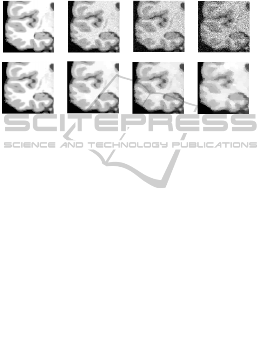
(a) Original phantom (b) Noisy for σ = 0.025 (c) Noisy for σ = 0.05 (d) Noisy for σ = 0.1
(e) Original phantom (f) Denoised for σ = 0.025, λ =
0.025
(g) Denoised for σ = 0.05, λ =
0.075
(h) Denoised for σ = 0.1, λ =
0.125
Figure 1: The original free noise phantom is shown in images a) and e). In b), c) and d) the contaminated phantoms for
σ = 0.025, 0.05 and 0.1 respectively. Below, their respective denoised images e), f) and g) for λ = 0.025, 0.075 and 0.125.
which is the Euler-Lagrange equation of the ROF en-
ergy functional ((Rudin et al., 1992)):
E(u) = |Du|(Ω) +
1
2β
Z
Ω
(u − g)
2
dx (16)
for β = σ
2
/(αλ) and g =
ˆ
f
n
, for any positive integer
n > 0, with (artificial) time t
n
= n∆t. Hence, at each
gradient descent step ∆t, we can solve a ROF problem
associated to the minimization of the energy (16) in
the space BV (Ω) ∩ [0, 1]. This problem is mathemat-
ically well-posed and it can be numerically solved by
very efficient methods, when formulated using well
known duality arguments (see (Chambolle, 2004) for
more details).
5 RESULTS AND DISCUSSION
The theoretical result presented in the previous sec-
tion have to be numerically confirmed in order to
asses the well behaviour of the method and also the
advantages it presents when it is compared to the orig-
inal regularized method which computes the approxi-
mating u
ε
solution. In order to assess the performance
of our algorithm we tested it with synthetic and real
brain images. The obtained results are presented and
discussed below.
Synthetic Brain Images
The synthetic brain images we used for our study
were obtained from the BrainWeb Simulated Brain
Database
1
at the Montreal Neurological Institute
(Aubert-Broche et al., 2006) . The original phantoms
were contaminated artificially with Rician noise con-
sidering the data as a complex image with zero imag-
inary part and adding random gaussian perturbations
to both the real and imaginary part, before comput-
ing the magnitude image. This process allows to con-
trol the amount and distribution of the Rician noise so
providing a gold standard for our study. For this we
used different values of the σ parameter which repre-
sents the variance of the noise (σ = 0.025, σ = 0.05
and σ = 0.1) and different values of the λ parame-
ter (λ = 0.05, λ = 0.1 and λ = 0.125). Notice that,
fixed σ (which can be estimated for real images) the λ
parameter is the only one we have to choose for regu-
larization (as in the gaussian case).
We can observe in Figure 1 the performance of
the denoising method based on the semi-implicit for-
mulation for λ = 0.05, λ = 0.1 and λ = 0.125. This
implicit method solves exactly the total variation op-
erator in (6) due to its dual formulation and not
its approximate form as the explicit method which
solves the primal formulation, so the solution ob-
tained should be close to the ideal minimum of (6).
This behaviour can be in fact observed in Figure 2,
where using the same values for the algorithms (∆t =
10
−3
and λ = 0.1) the proposed method reach a solu-
tion whose energy is smaller than the obtained by the
solution of the first method. This difference caused
by the fact that now we are using the true Total Vari-
1
available at http://www.bic.mni.mcgill.ca/brainweb
BIOSIGNALS 2012 - International Conference on Bio-inspired Systems and Signal Processing
18
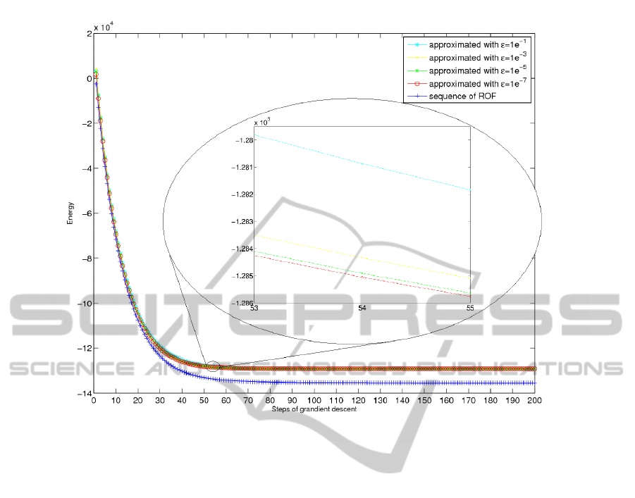
Figure 2: Energy in functional 6 of the solution obtained at each step of the gradient descent by the approximated method
for λ = 0.1, σ = 0.05, dt = 0.001 and different values of ε = 10
−1
,10
−3
,10
−5
,10
−7
, and by the new method for λ = 0.1,
σ = 0.05, dt = 0.001.
ation can be also observed in the images of the ab-
solute difference between the original (free of noise)
image and the solutions found by the two methods.
We can see how the image difference corresponding
to the solution of the approximated method ( Figure
3 a ) presents more structural details than the image
corresponding to the implicit method ( Figure 3 b ),
which confirms that this last method recovers more
structural details, that are eventually lost by the ex-
plicit method because of the ε approximation.
The other important characteristic of this new for-
mulation is that the diffusion term is implicitly con-
sidered and this provides numerical stability which
in turn allows to increase the value of ∆t compared
to those used in the explicit method, so less itera-
tions of the algorithm are necessary for time stabi-
lization. In fact if we increase the value of ∆t to
the value ∆t = 10
−1
the explicit method becomes un-
stable and it begins to oscillate without reaching the
minimum of the energy we obtained with ∆t = 10
−3
.
Also the implicit method takes less iterations to reach
the same minimum. The performance of the two al-
gorithms for ∆t = 10
−1
can be observed in Figure 4
where the energy computed along the iterates of the
implicit method is clearly less than the same energy
calculated along the approximated iterates.
This behaviour is crucial for the selection of the
algorithm in so far even if the new method has more
computational cost per iteration (because we solve a
ROF problem at each iteration), we can increase the
value of ∆t in order to reach the solution in less it-
erations than the first method, finding a best solution
for our problem (in the sense of figure 4) and spend-
ing less time of computation. Finally, in the last fig-
ure(figure 5) we show that this framework is robust
in the sense that the same solution is obtained when
completely different initial condition are used for ini-
tialization in the gradient flow schemes we consid-
ered. This is suggestive of uniqueness for the non
trivial solution of the corresponding elliptic problems.
Real Brain Images
Apart from the modelling exercise and the imple-
mentation details of the algorithm presented above,
our main interest relies in the application of the pro-
posed algorithm to real brain images. In the following
we present some preliminary results we are obtaining
for Diffusion Weighted Magnetic Resonance Images
(DW-MRI) denoising. The DW-MR images are ac-
quired and used for Diffusion Tensor Image (DTI) re-
AN EFFICIENT NUMERICAL RESOLUTION FOR MRI RICIAN DENOISING
19
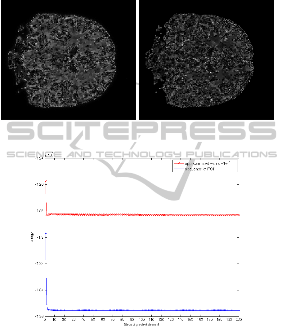
(a) Existing method (b) Proposed method
Figure 3: Absolute difference between the original image and the solution of the existing method and the proposed method
for the values λ = 0.1, σ = 0.05, dt = 0.001 in both methods and ε = 10
−
7 for the approximated method.
Figure 4: Energy in functional 6 of the solution obtained at each step of the gradient descent by the approximated method for
ε = 10
−7
, λ = 0.1, σ = 0.05, dt = 0.1 and by the new method for λ = 0.1, σ = 0.05, dt = 0.1.
construction, and the importance of the denoising step
is crucial in DW-MRI analysis because their charac-
teristic very low SNR (Basu et al., 2006). Diffusion
Tensor Imaging is a MRI technique that can mea-
sure the water diffusion which is restricted by the sur-
rounding structure, and this allows to infer the macro-
scopic axonal organization in nervous system tissues.
We show the results of the DTI reconstruction for
BIOSIGNALS 2012 - International Conference on Bio-inspired Systems and Signal Processing
20
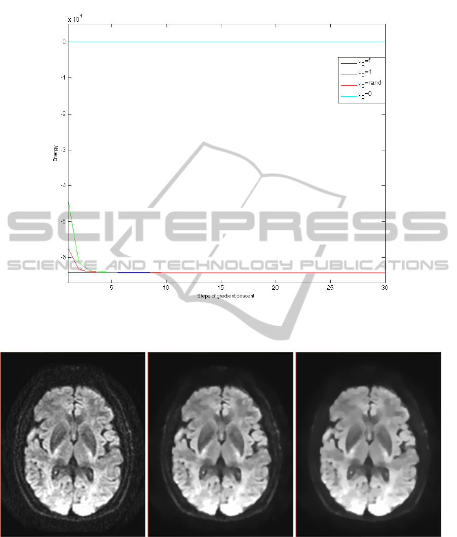
Figure 5: Energy in functional 6 of the solution obtained at each step of the gradient descent by the new method for λ = 0.05,
σ = 0.05, dt = 0.1 and different initial data u
0
: black image (u
0
≡
¯
0), white image (u
0
≡
¯
1), the noisy image (u
0
≡ f ) and a
random image (u
0
≡ rand).
(a) Original (b) Denoised with λ = σ/2 (c) Denoised with λ = σ/4
Figure 6: A slice of the original Diffusion Weighted Image corresponding to the (1, 0, 0) gradient direction and the corre-
sponding denoised images.
the original DW-MRI data and the correspondent de-
noised data with different values of the parameter λ.
For this preliminary study we have used a
DW-MR brain volume provided by Fundaci
´
on
CIEN-Fundaci
´
on Reina Sof
´
ıa which was acquired
with a 3 Tesla General Electric scanner equipped
with an 8-channel coil. The DW images have
been obtained with a single-shot spin-eco EPI
sequence (FOV=24cm, TR=9100, TE=88.9, slice
thickness=3mm, spacing=0.3, matrix size=128x128,
AN EFFICIENT NUMERICAL RESOLUTION FOR MRI RICIAN DENOISING
21
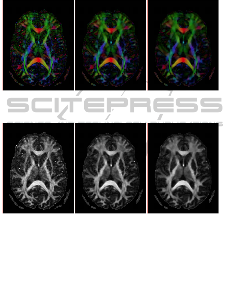
(a) From original DWI data (b) From denoised DWI data with λ = σ/2 (c) From denoised DWI data with λ = σ/4
Figure 7: A slice of the colormap orientation (of the main eigenvector) of the DTI data. red means right-left direction, green
anterior-posterior and blue inferior-superior. Fibers with an oblique angle have a color that is a mixture of the principal colors
and black color is used for the isotropic regions as the cerebrospinal fluid.
(a) From original DWI data (b) From denoised DWI data with λ = σ/2 (c) From denoised DWI data with λ = σ/4
Figure 8: A slice of the Fractional Anisotropy estimated from the Tensor Image. Dark colour corresponds to values near zero
(isotropic regions) and bright color corresponds to values near one (anisotropic regions).
NEX=2 ). The DW-MRI data consists on a vol-
ume obtained with b=0/mm
2
and 15 volumes with
b=1000s/mm
2
corresponding with the gradient direc-
tions specified in (DK Jones, 1999). These DW-
MR images, which represent diffusion measurements
along multiples directions, are denoised with the pro-
posed method previously to the Diffusion Tensorial
Image reconstruction, which was done with the 3d
Slicer tools
2
.
In Figure 6(a) we show a slice of the original DWI
2
Free available in http://www.slicer.org/
data corresponding to the (1, 0, 0) gradient direction
where the affecting noise is clearly visible. The com-
plete DW-MRI data volume is denoised using the pro-
posed method where the Rician noise magnitude (σ)
has been estimated for each gradient direction follow-
ing (Sijbers et al., 1998), while we have used two
different values of λ for the denoising, λ = σ/2 and
λ = σ/4. The two slices resulting from the denoising
process are shown in Figures 6(b) and 6(c). It can be
observed that smaller values of λ provide stronger dif-
fusion (which is coherent with the model formulation
in 6) and how in the two denoised images the noise
BIOSIGNALS 2012 - International Conference on Bio-inspired Systems and Signal Processing
22

has been removed but the details and the edges have
been fully preserved, as we should expect when the
exact TV model is solved.
The effect of this denoising process over the re-
constructed tensor and their derived scalar measure-
ments (obtained with the 3d Slicer tools) is presented
in Figures 7 and 8. Figure 7 shows a color-coded
orientation map created from DTI data. In this im-
age, the principal colors (red, green, and blue) rep-
resent fibers running along the spatial orientations
(x,y, z). Results in 7 shows that the structures are
better defined if the DW-MRI volume is denoised
previously. As evidenced by Figure 8 this effect is
yet more visible in the measurements like the Frac-
tional Anisotropy where the structures and details are
clearly enhanced. When we use a lower value for λ
(Figures 7(c) and 8(c)) we obtain smoother tensorial
images but some details can be better distinguished
when the value of λ is higher (Figures 7(b) and 8(b)).
6 CONCLUSIONS
In this notes we address the problem of the numeri-
cal computation of the solution of the variational for-
mulation of the Rician denoising model proposed in
(Mart
´
ın et al., 2011). We deduce a semi-implicit for-
mulation for the gradient flow which leads to the res-
olution of ROF like-problems at each step of the time
discretization. This is accomplished efficiently using
a gradient descent for the dual variable associated to
the primal ROF model. While our study is prelim-
inary it indicates how to obtain fast numerical solu-
tions for Rician denoising. This is specially inter-
esting when Diffusion Wheighted Images (DWI) are
considered for Diffusion Tensor Images reconstruc-
tion whereas they have poor resolution and low SNR
which makes Rician denoising necessary.
Challenging mathematical issues arise about the
existence, uniqueness and convergence, when ε → 0,
of weak bounded variation solutions of the quasilinear
elliptic equations considered in this paper (i.e. (8) and
(12)) and the gradient flow analysis of their parabolic
counterpart ((10) and (13)) when t → +∞. A rigor-
ous justification of the above arguments is desired.
Nevertheless this approach is the mostly used regu-
larization technique to approximate and compute the
minimizer of the total variation energy and its variants
(see (Casas et al., 1998)).
The semi-implicit method we propose is well
founded mathematically when the time-discretized
problems are dealt with and it represents a feasible al-
ternative to gaussian denoising for low SNR MR im-
ages. Further study is undoubtedly necessary in order
to make automatic the choice of the parameters in real
medical images. Other possibilities, such as Inverse
scaling, which makes the parameter estimation less
crucial and provide contrast enhanced images shall
also be explored.
ACKNOWLEDGEMENTS
This work was supported by project TEC2009-14587-
C03-03 of the Spanish Ministry of Science. Also we
thank to Mrs. Eva Alfayate, MR-scanner technician
of the Fundaci
´
on Reina Sof
´
ıa, for her professional and
kindly collaboration.
REFERENCES
Ambrosio, L., Fusco, N., and Pallara, D. (2000). Functions
of Bounded Variation and free discontinity problems.
The Clarendon Press, Oxford University.
Aubert-Broche, B., Griffin, M., Pike, G., Evans, A., and
Collins, D. (2006). Twenty new digital brain phan-
toms for creation of validation image data bases. In
IEEE transactions on Medical Imaging, volume 25,
pages 1410–1416.
Basu, S., Fletcher, T., and Whitaker, R. (2006). Rician
noise removal in diffusion tensor mri. Medical Im-
age Computing and Computer-Assisted Intervention,
9(Pt 1):117–125.
Casas, E., Kunisch, K., and Pola, C. (1998). Some applica-
tions of bv functions in optimal control and calculus
of variations. In ESAIM: Proceedings. Control and
partial differential equations, volume 4, pages 83–96.
Chambolle, A. (2004). An algorithm for total variation
minimization and applications. Journal Mathematical
Imaging and Vision, 20:89–97.
DK Jones, MA Horsfield, A. S. (1999). Optimal strate-
gies for measuring diffusion in anisotropic systems
by magnetic resonance imaging. Journal of Magnetic
Resonance in Medicine, 42 (3):515–525.
Gudbjartsson, H. and Patz, S. (1995). The rician distribution
of noisy mri data. Magnetic Resonance in Medicine,
34(6):910–914.
Henkelman, R. M. (1985). Measurement of signal intensi-
ties in the presence of noise in mr images. Medical
Physics, 12(2):232–233.
Lassey, K. R. (1982). On the computation of certain in-
tegrals containing the modified bessel function i
0
(ξ).
Mathematics of Computation, 39.
Lysaker, M., Lundervold, A., and cheng Tai, X. (2003).
Noise removal using fourth-order partial differential
equations with applications to medical magnetic res-
onance images in space and time. IEEE Trans. Imag.
Proc, 12:1579–1590.
Mart
´
ın, A., Garamendi, J., and Schiavi, E. (2011). Iterated
rician denoising. In IPCV’11 Proceedings, Las Vegas,
Nevada, USA. CSREA Press.
AN EFFICIENT NUMERICAL RESOLUTION FOR MRI RICIAN DENOISING
23

Nikolova, M., Esedoglu, S., and Chan, T. F. (2006). Al-
gorithms for finding global minimizers of image seg-
mentation and denoising models. SIAM Journal of Ap-
plied Mathematics, 66(5):1632–1648.
Perona, P. and Malik, J. (1990). Scale-space and edge de-
tection using anisotropic diffusion. Pattern Analy-
sis and Machine Intelligence, IEEE Transactions on,
12(7):629–639.
Rudin, L. I., Osher, S., and Fatemi, E. (1992). Nonlinear to-
tal variation based noise removal algorithms. Physica
D Nonlinear Phenomena, 60:259–268.
Sijbers, J., Dekker, A. D., Audekerke, J. V., Verhoye, M.,
and Dyck, D. V. (1998). Estimation of the noise in
magnitude mr images. Magnetic Resonance Imaging,
1(16):87–90.
BIOSIGNALS 2012 - International Conference on Bio-inspired Systems and Signal Processing
24
