
TISSUE TYPE DIFFERENTIATION FOR BRAIN
GLIOMA USING NON-NEGATIVE MATRIX FACTORIZATION
Yuqian Li
1,2,3
, Diana M. Sima
2,3
, Sofie Van Cauter
4,5
, Uwe Himmelreich
5
, Yiming Pi
1
and Sabine Van Huffel
2,3
1
School of Electronic Engineering, University of Electronic Science and Technology of China
Xiyuan Dadao 2006, Chengdu, China
2
Department of Electrical Engineering, ESAT-SCD, Katholieke Universiteit Leuven, Leuven, Belgium
3
IBBT-K.U.Leuven Future Health Department, Leuven, Belgium
4
Department of Radiology, University Hospitals of Leuven, Leuven, Belgium
5
Biomedical NMR Unit/Molecular Small Animal Imaging Center, Department of Medical Diagnostic Sciences
Katholieke Universiteit Leuven, Leuven, Belgium
Keywords: Non-negative Matrix Factorization (NMF), Blind Source Separation (BSS), Magnetic Resonance
Spectroscopic Imaging (MRSI), Brain Glioma, Glioblastoma Multiforme (GBM).
Abstract: The purpose of this paper is to introduce a hierarchical Non-negative Matrix Factorization (NMF) approach,
customized for the problem of blindly separating brain glioma tumor tissue types using short-echo time
proton magnetic resonance spectroscopic imaging (
1
H MRSI) signals. The proposed algorithm consists of
two levels of NMF, where two constituent spectra are computed in each level. The first level is able to
correctly detect the spectral profile corresponding to the most predominant tissue type, i.e., normal tissue,
while the second level is optimized in order to detect two ‘abnormal’ spectral profiles so that the 3
recovered spectral profiles are least correlated with each other. The two-level decomposition is followed by
the reestimation of the overall spatial distribution of each tissue type via standard Non-negative Least
Square (NNLS). This method is demonstrated on in vivo short-TE
1
H MRSI brain data of a glioblastoma
multiforme patient and a grade II-III glioma patient. The results show the possibility of differentiating
normal tissue, tumor tissue and necrotic tissue in the form of recovered tissue-specific spectra with accurate
spatial distributions.
1 INTRODUCTION
Glioblastoma multiforme (GBM), which is the
highest grade of glioma, is the most common and
aggressive type of brain tumor in adults. Accurate
diagnosis is of utmost importance in guiding therapy
and determining prognosis. Magnetic resonance
spectroscopic imaging (MRSI) (
Brown et al.,
1982
), which provides both spectral and spatial
information, is becoming increasingly popular as an
additional non-invasive tool for clinical diagnosis of
brain tumors. Since the concentration of metabolites
changes under disease conditions, the profile of the
measured signal in each MRSI voxel helps to
determine the location of abnormal tissue (Howe et
al., 2003).
Because of the heterogeneity of GBMs, the
tumoral region could consist of several tissue types
(Croitor Sava et al., 2011), which represent actively
growing tumor, necrosis or normal brain tissue.
Lower grade gliomas do not contain necrosis, but are
also heterogeneous, e.g., the tumor can present
infiltrations into the normal brain tissue. In MRSI,
the partial volume effect, i.e., the presence of several
tissue types within one voxel, may lead to increased
variability in the measured signals. The spectrum
corresponding to each voxel can be approximately
described as a linear combination of spectra from
different constituent tissue types (Su et al., 2008).
Using Non-negative matrix factorization (NMF)
to extract main tissue types from the mixed MRSI
data was firstly proposed by Sajda and his
colleagues (Sajda et al., 2003; Sajda et al., 2004; Du
25
Li Y., Sima D., Van Cauter S., Himmelreich U., Pi Y. and Van Huffel S..
TISSUE TYPE DIFFERENTIATION FOR BRAIN GLIOMA USING NON-NEGATIVE MATRIX FACTORIZATION.
DOI: 10.5220/0003734600250031
In Proceedings of the International Conference on Bio-inspired Systems and Signal Processing (BIOSIGNALS-2012), pages 25-31
ISBN: 978-989-8425-89-8
Copyright
c
2012 SCITEPRESS (Science and Technology Publications, Lda.)
et al., 2008; Su et al., 2008). They developed a
constraint NMF (cNMF) algorithm, which enforces
positivity, and incorporate it into a hierarchical
decomposition framework to recover physically
meaningful spectra using long echo time (TE) MRSI
signals.
In this paper, we study the applicability of a
novel hierarchical NMF method for tissue type
differentiation on short-TE MRSI data, which is
potentially much more challenging than long-TE due
to more complex spectral profiles. The proposed
algorithm, as described in Section 3, consists of two
levels of NMF, where two constituent spectra are
computed in each level. Thus, we recover each
tissue type step by step using NMF, i.e., first
differentiate normal and abnormal tissue, and then,
only in the abnormal region, differentiate active
tumor and necrosis, or differentiate proliferation
level of active tumor if necrosis is not present. Since
the choice of the abnormal region has a high
influence on the estimated sources, we propose to
tune the threshold for selecting the abnormal region
by minimizing the correlations between all three
estimated tissue spectra, i.e., normal tissue spectral
profile from the first-level NMF, and the two
abnormal spectral profiles from the second-level
NMF. Afterwards, non-negative least squares
(NNLS) is applied on the original mixed signals
using the obtained spectra in order to reestimate the
spatial distribution of each tissue type over the
whole grid. In section 4, experimental results on two
typical patients show the capability of revealing
tissue-specific spectral profiles and their spatial
distribution, and are validated against expert
labelling.
2 IN VIVO 1H MRSI DATA
2.1 Data Acquisition Protocol and
Patients
The short-TE MRSI data were acquired at the
University Hospital of Leuven (UZ Leuven) on a 3T
MR scanner (Achieva, Philips, Best, The
Netherlands). Point-resolved spectroscopy (PRESS)
(Bottomley, 1987) was used as the volume selection
technique, TR/TE: 2000/35 ms, FOV: 16cm*16 cm,
volume of interest (VOI): 8cm*8cm, slice thickness:
1cm, acquisition voxel size: 1cm*1cm,
reconstruction voxel size: 0.5cm*0.5 cm, receiver
bandwidth: 2000Hz, samples: 2048.
Our algorithm was tested on two types of
patients:
In vivo MRSI data of GBM patients containing
necrotic areas. Anatomic image of a typical
patient is shown in Figure. 1(a)
In vivo MRSI data of glioma patients with no
apparent necrotic area. Figure 1 (b) shows the
anatomic image of a typical patient who has a
grade Ⅱ glioma with focal progression to a
grade Ⅲ glioma.
(a)
(b)
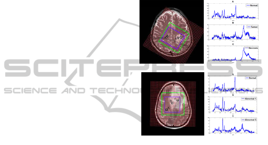
Figure 1: Left: Anatomic image. Right: tissue specific
spectra of patients. (a) Patient 1, a GBM patient with
necrosis. (b) Patient 2, a glioma patient with no apparent
necrosis areas. The outer green box is the PRESS box and
the inner blue box contains the selected voxels of interest.
2.2 Data Preprocessing
In-house software SPID (Poullet, 2008), which was
developed on the Matlab platform, was used for
standard spectroscopic signal preprocessing. The
applied steps were as follows:
In the MRSI grid, signals of insufficient quality
(low signal-to-noise ratio (SNR), baseline
problems, chemical shift displacement effects,
etc.) usually exist, affecting mostly the voxels
close to the border of the PRESS box. Therefore,
these signals were excluded by selecting an inner
smaller box inside the PRESS box of the MRSI
grid (see Fig.1).
Residual water components ware removed using
Hankel-Lanczos Singular Value Decomposition
with Partial Re-Orthogonalization (HLSVD-
PRO) (Laudadio et al., 2002). The model order
BIOSIGNALS 2012 - International Conference on Bio-inspired Systems and Signal Processing
26

was set to 30 and the passband from 0.25 to 4.2
ppm.
A baseline offset correction was found
necessary. But this is not suppressing the
baseline due to macromolecules, which may be
relevant for tissue differentiation.
The real parts of the preprocessed spectra were
truncated to the region 0.25 – 4.2 ppm before
analyzing them using the NMF algorithm.
3 METHODS
3.1 Basics of Non-negative Matrix
Factorization (NMF)
NMF (Paatero et al., 1994; Lee et al., 1999), as a
blind source separation (BSS) method, has attracted
much attention in performing the factorization:
XWHN=+
(1)
where
X
is a matrix of observed MRSI spectra
represented as column vectors, with one column per
voxel.
W
is a matrix of constituent tissue spectra,
with each column representing a typical spectrum
for each tissue type. Each row of the matrix
H
contains the linear combination weights (interpreted
here as abundances or concentrations) of all
constituent tissue spectra.
N
stands for additive
measurement noise. The mathematical formulation
of the basic NMF problem is
2
,
1
min ( , ) || ||
2
0, 0
F
WH
fWH X WH
subject to W H
=−
≥≥
(2)
3.2 Hierarchical NMF-NNLS
In this section, a hierarchical NMF-NNLS algorithm,
which recovers the 3 most distinct tissue-specific
spectral profiles and their corresponding spatial
distributions step by step, is described.
Step 1: First level NMF
. Apply NMF to the
preprocessed MRSI signals with the number of
components chosen to be 2. Two patterns of
spectra (W-normal and W-abnormal,
respectively) and their contribution to each
location in the brain image (H-normal and H-
abnormal) will be recovered. Then, label the
obtained 2 sources as normal and abnormal
tissue types according to typical metabolic
features of their spectral profiles (i.e., the NAA
peak at 2.01 ppm is higher in the source
corresponding to normal tissue).
Step 2: Automatically find the optimal threshold
for the abnormal region. Perform intermediate
NMF decompositions with 2 sources on
gradually increasing sets of voxels, where these
sets are selected according to a variable threshold
on the magnitude of the H-abnormal map. A
reasonable trade-off for mutually least
correlation between recovered spectral profiles is
found by minimizing the sum: Corr(W-
normal,W-abnormal1) + Corr(W-normal,W-
abnormal2) + Corr(W- abnormal1+W-
abnormal2).
Step 3: Second level NMF
. Apply NMF only to
the voxels of the abnormal region selected using
the optimal threshold in order to further separate
the abnormal tissue into two abnormal tumor
profiles, which reflect the aggressiveness level,
with their corresponding spatial distributions. If
one of the profiles contains predominantly lipids
(according to the peaks at 0.9 and 1.3 ppm) and
almost no other metabolites, then label that
profile as necrosis.
Step 4: NNLS reestimation
. Since the second
level NMF was restricted to the selected
abnormal region, some border voxels containing
abnormal tissue may have been excluded due to
the thresholding. Applying non-negative least
squares approach (Lawson et al., 1974) to the
whole grid with the 3 recovered tissue spectra
(i.e., solving problem [2] for W fixed to a three-
column matrix [W-normal, W-abnormal1, W-
abnormal2]) will give a complete estimation of
the spatial information of these 3 tissue types
over the whole initially considered grid.
4 EXPERIMENTAL RESULTS
We studied the applicability of brain tumor tissue
type differentiation using the proposed hierarchical
NMF-NNLS algorithm. The results of two different
cases are shown in Figure 2 and Figure 3.
4.1 Results for Patient 1: GBM Patient
with Necrosis
Results of 2-level hierarchical NMF-NNLS to the
preprocessed brain signals of patient 1 are shown in
Figure 2. The corresponding anatomic picture of the
patient 1 (male, GBM) is shown in Figure 1 (a) with
the green box and the blue box representing the
TISSUE TYPE DIFFERENTIATION FOR BRAIN GLIOMA USING NON-NEGATIVE MATRIX FACTORIZATION
27
PRESS box and the selected voxels of reasonable
quality, respectively. Figure 2 (a) presents the
recovered normal and abnormal spectra of the first
level NMF. The spectrum that shows a decreased
NAA/Cho ratio, a decreased Cre and significant
levels of Lac-Lip, represents the tumor tissue. The
one with almost no metabolites other than lipids
(and potentially lactate), is the typical spectral
pattern of necrotic tissue. The H-maps in (b) give
their spatial distribution. (c) illustrates the selected
abnormal region. (d) and (e) are the results of the
second level NMF. (f) shows the reestimated spatial
information using NNLS. We can see tumor and
necrosis in (c) covering bigger regions than in (b)
and therefore being able to show more complete
information at the border region which contains
mixed tissues.
4.2 Results on Glioma Patients with no
Apparent Necrosis Area
To explore the applicability of the proposed method
(see Section 2.4), it was tested on another case,
which is a patient who has been diagnosed with
grade II-III glioma and, according to the expert
labeling, does not present macroscopic necrosis;
Anatomic picture is given in Figure 1 (b). Results
are shown in Figure 3. It is controversial if we still
try to search for 3 components with our method
when there is no necrosis. Still, this situation is
realistic, because in most cases we are not sure
beforehand if there is necrosis within the lesion.
Figure 3 (a) and (b) give the results of the first level
decomposition and thresholding. Panel (a) illustrates
the recovered spectra of normal tissue and abnormal
tissue; the H-maps in (b) show the spatial
distribution of the corresponding spectra after
Figure 2: Result of hierarchical NMF-NNLS on patient 1, a GBM patient with necrosis. (a) – (b): Step 1, first level NMF.
(c): Abnormal region after optimal thresholding. (d) – (e): Step 3, second level NMF. (f): Step 4, NNLS.
BIOSIGNALS 2012 - International Conference on Bio-inspired Systems and Signal Processing
28
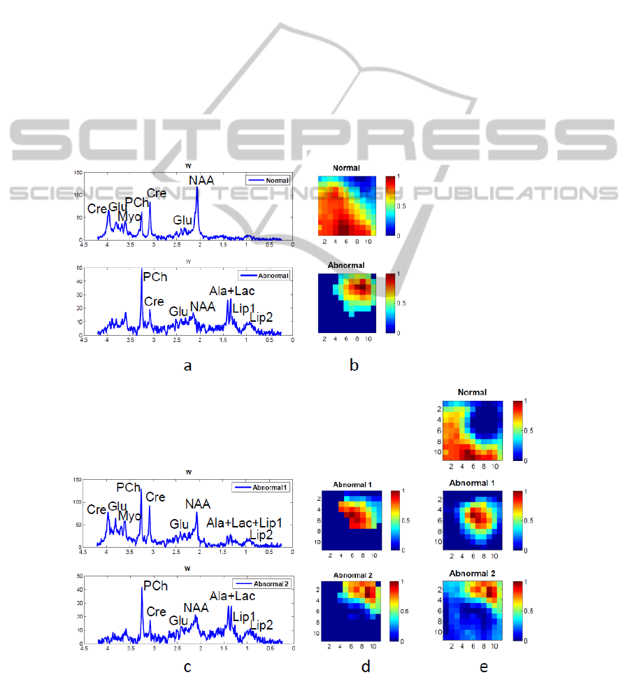
thresholding. We can see that the factorization is
effective in finding normal and abnormal tissue.
Then, in Step 3, the abnormal tissue was
separated into two parts that apparently do not
contain necrotic tissue (also confirmed by the
absence of lipids). The one near the normal region is
the border of the tumor, with its spectral pattern
(Abnormal 1 in Figure 3 (c)) still indicating
abnormality (low NAA/Cho). The recovered
spectrum from the other part of abnormal region
(Abnormal 2 in Figure 3 (c)) has a significant
increase of Cho and Lips, obvious peaks of Ala and
Lac, and a decrease of other metabolites. For this
case without necrosis, instead of separating tumor
and necrosis, our proposed method reveals the
regions in the tumor that correspond to different
levels of proliferating tumor cells. In the end, NNLS
estimation gives more complete spatial information
of each tissue type.
4.3 Results Validation
The distribution maps of the 3 tissue types were
overlapped onto the anatomical images; see Fig. 4.
The recovered location of our results corresponds
well to the one shown on the anatomic image.
As an additional validation for patient 1, we also
computed correlation coefficients between the
recovered spectra and the average of pure tissue-
specific spectra according to the labeling of an
expert (SVC). The result for normal tissue is 0.9933,
for tumor is 0.9618 and for necrosis is 0.9950, which
shows that all spectral sources are relatively highly
correlated with the validated spectra.
For patient 2, who has grade II-III glioma but
without macroscopic necrosis, the result of our
proposed method reflected the level of tumour
proliferation, which was validated by histopathology.
Figure 3: Result of hierarchical NMF-NNLS on patient 2, a glioma patient with no apparent necrosis area. (a) – (b): Step 1-
2, first level NMF and optimally selected abnormal region (c) – (d): Step 3, second level NMF. (e): Step 4, NNLS.
TISSUE TYPE DIFFERENTIATION FOR BRAIN GLIOMA USING NON-NEGATIVE MATRIX FACTORIZATION
29
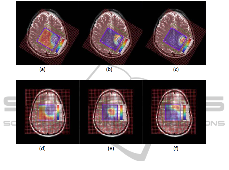
Figure 4: Overlap of the distribution results onto the anatomic images. The first row is the result of the GBM patient with
necrosis. (a): normal tissue distribution; (b): tumor tissue distribution; (c): necrosis tissue distribution. The second row is the
result of the glioma patient without necrosis. (a): normal tissue distribution; (b): abnormal 1 tissue distribution; (c):
abnormal 2 tissue distribution.
5 DISCUSSION & CONCLUSIONS
A novel tissue type differentiation approach,
hierarchical NMF-NNLS, and its clinical application
were explored in this study for GBM patients.
The data we used in this study is short-TE MRSI
signals because spectra of short-TE represent more
metabolites than long-TE spectra. But there is more
significant peak overlap and, usually, a higher noise
level. Therefore, using short-TE signals in solving
tissue type differentiation is more challenging but of
more significance.
The reason we need the hierarchical procedure is
based on the assumption in the considered data sets
that the MRSI grid encompasses mostly normal
tissue and a glioma tumor with heterogeneous tissue
content. Due to the unbalanced proportion of the
tumor tissue voxels inside the grid, the sources
corresponding to under-represented tissue types
would be difficult to be identified by simply using
NMF with more than 2 sources. Therefore, the
robustness of NMF for extracting meaningful
spectral patterns can be increased through a
hierarchical NMF approach.
The possibility of differentiating brain tumor
tissue types was demonstrated in two distinct cases.
Representative results from a GBM patient showed
the capability of the proposed algorithm to separate
short-TE MRSI data into normal tissue, tumor and
necrosis with accurate spatial information. For the
case of a glioma patient without necrosis, our
method is able to indicate the proliferation level of
the tumor. This result is useful because assessing
tumor proliferation level is important in brain tumor
diagnosis, as it gives information that is potentially
helpful in directing the patient’s clinical
management. Both cases show that the proposed
method is able to find meaningful sources and their
corresponding spatial distributions using short-TE
MRSI signals.
However, the data presented in this paper is
preliminary and a more appropriate data pool will be
BIOSIGNALS 2012 - International Conference on Bio-inspired Systems and Signal Processing
30

used in future work in order to actually fully assess
the performance of the proposed technique.
Another paper appearing in these proceedings
focuses on a “simulation study of tissue type
differentiation using non-negative matrix
factorization”. In that preliminary research, we
studied the performance of several NMF
implementations on simulated MRSI signals. The
‘(a)hals’ algorithm (Cichocki et al., 2007; Cichocki
et al., 2009; Gillis, 2011) had the best performance
in those simulations and has therefore been used for
all the NMF computations in this paper.
ACKNOWLEDGEMENTS
This research was supported by Research Council
KUL: GOA MaNet, CoE EF/05/006 Optimization in
Engineering (OPTEC), PFV/10/002 (OPTEC), IDO
08/013 Autism, several PhD/postdoc & fellow grants;
Flemish Government: FWO: PhD/postdoc grants,
projects: FWO G.0302.07 (SVM), G.0341.07 (Data
fusion), G.0427.10N (Integrated EEG-fMRI),
G.0108.11 (Compressed Sensing) research
communities (ICCoS, ANMMM); IWT:
TBM070713-Accelero, TBM070706-IOTA3,
TBM080658-MRI (EEG-fMRI), PhD Grants; IBBT
Belgian Federal Science Policy Office: IUAP P6/04
(DYSCO, `Dynamical systems, control and
optimization', 2007-2011); ESA AO-PGPF-
01, PRODEX (CardioControl) C4000103224;
EU: RECAP 209G within INTERREG IVB NWE
programme, EU HIP Trial FP7-HEALTH/ 2007-
2013 (n° 260777) (Neuromath (COST-BM0601):
BIR&D Smart Care. Li thank the China Scholarship
Council.
REFERENCES
Bottomley PA, 1987. Spatial localization in NMR-
spectroscopy in vivo. Ann N Y Acad Sci, 508:333–348.
Brown T, Kincaid B, Ugurbil K, 1982. NMR chemical
shift imaging in three dimensions. PNAS, 79(11):
3523-3526.
Croitor Sava A, Martinez-Bisbal MC, Van Huffel S, Cerda
JM, Sima DM, Celda B, 2011. Ex vivo high resolution
magic angle spinning metabolic profiles describe
intratumoral histopathological tissue properties in
adult human gliomas. Magn Reson Med, 65:320-328.
Cichocki A, Zdunek R, Amari S, 2007. Hierarchical ALS
algorithms for nonnegative matrix and 3D tensor
factorization. Lect Notes Comput Sci, 4666:169-176.
Cichocki A, Phan AH, 2009. Fast local algorithms for
large scale Nonegative Matrix and Tensor
Factorizations. IEICE Trans Fund Electron Comm
Comput Sci, 3:708-721.
Du S, Mao X, Sajda P and Shungu DC, 2008. Automated
tissue segmentation and blind recovery of 1H MRS
imaging spectral patterns of normal and diseased
human brain. NMR in Biomedicine, 21:33-41.
Gillis N, 2011. Nonnegative matrix factorization
complexity, algorithms and applications. PhD Thesis,
Louvan-La-Neuve, Belgium.
Howe FA, Barton SJ, Cudlip SA, Stubbs M, Saunders DE,
Murphy JR, Opstad KS, Doyle VL, McLean MA, Bell
BA, Griffiths JR, 2003. Metabolic profiles of human
brain tumours using quantitative in vivo 1H magnetic
resonance spectroscopy. Magn Res Med, 49:223-232.
Laudadio T, Mastronardi N, Vanhamme L, Van Hecke P,
Van Huffel S, 2002. Improved Lanczos algorithms for
blackbox MRS data quantitation. J Magn Reson, 157:
292-297.
Lawson C.L. and R.J. Hanson, 1974, Solving Least-
Squares Problems, Prentice-Hall, Chapter 23, p. 161,.
Lee DD, Seung HS, 1999. Learning the parts of objects by
non-negative matrix factorization. Nature, 401:788-
791.
Paatero P, Tapper U, 1994. Positive matrix factorization:
A non-negative factor model with optimal utilization
of error. Environmetrics, 5:111-126.
Poullet JB, 2008. Quantification and classification of
magnetic resonance spectroscopic data for brain
tumor diagnosis. PhD Thesis, Leuven, Belgium.
Sajda P, Du S, Brown TR, Parra LC, Stoyanova R, 2003.
Recovery of constituent spectra in 3D chemical shift
imagin using non-negative matrix factorization. In
Proc. 4th Int. Symp. ICA and BSS, 71-76.
Sajda P, Du S, Brown TR, Stoyanova R, Shungu DC, Mao
X, Parra LC, 2004. Nonnegative Matrix Factorization
for Rapid Recovery of Constituent Spectra in
Magnetic Resonance Chemical Shift Imaging of the
Brain. IEEE Trans Med Imaging, 23:1453-1465.
Su Y, Thakur SB., Karimi S, Du S, Sajda P, Huang W,
Parra LC, 2008. Spectrum separation resolves partial-
volume effect of MRSI as demonstrated on brain
tumor scans. NMR Biomed, 21:1030-1042.
TISSUE TYPE DIFFERENTIATION FOR BRAIN GLIOMA USING NON-NEGATIVE MATRIX FACTORIZATION
31
