SIMULATION STUDY OF TISSUE TYPE DIFFERENTIATION
USING NON-NEGATIVE MATRIX FACTORIZATION
Yuqian Li
1,2,3
, Diana M. Sima
2,3
, Sofie Van Cauter
4,5
, Uwe Himmelreich
5
, Yiming Pi
1
and Sabine Van Huffel
2,3
1
School of Electronic Engineering, University of Electronic Science and Technology of China,
Xiyuan Dadao 2006, Chengdu, China
2
Department of Electrical Engineering, ESAT-SCD, Katholieke Universiteit Leuven, Leuven, Belgium
3
IBBT-K.U.Leuven Future Health Department, Leuven, Belgium
4
Department of Radiology, University Hospitals of Leuven, Leuven, Belgium.
5
Biomedical NMR Unit/Molecular Small Animal Imaging Center, Department of Medical Diagnostic Sciences,
Katholieke Universiteit Leuven, Leuven, Belgium
Keywords: Glioma, Magnetic Resonance Spectroscopic Imaging (MRSI), Non-negative Matrix Factorization (NMF),
Blind Source Separation (BSS).
Abstract: Finding the brain tumor tissue-specific magnetic resonance spectra and their corresponding spatial
distribution is a typical Blind Source Separation (BSS) problem. Non-negative Matrix Factorization (NMF),
which only requires non-negativity constraints, has become popular because of its advantages compared to
other BSS methods. A variety of algorithms based on traditional NMF have been recently proposed. This
study focuses on the performance comparison of several NMF implementations, including some newly
released methods, in brain glioma tissue differentiation using simulated magnetic resonance spectroscopic
imaging (MRSI) signals. Experimental results demonstrate the possibility of finding typical tissue types and
their distributions using NMF algorithms. The (accelerated) hierarchical alternating least squares algorithm
was found to be the most accurate.
1 INTRODUCTION
Automatic tissue type differentiation in brain tumor
patients is of utmost importance in guiding therapy
and determining prognosis. Magnetic resonance
spectroscopic imaging (MRSI) (Brown et al., 1982),
which produces localized spectra, is used as a non-
invasive tool for additional clinical diagnosis of
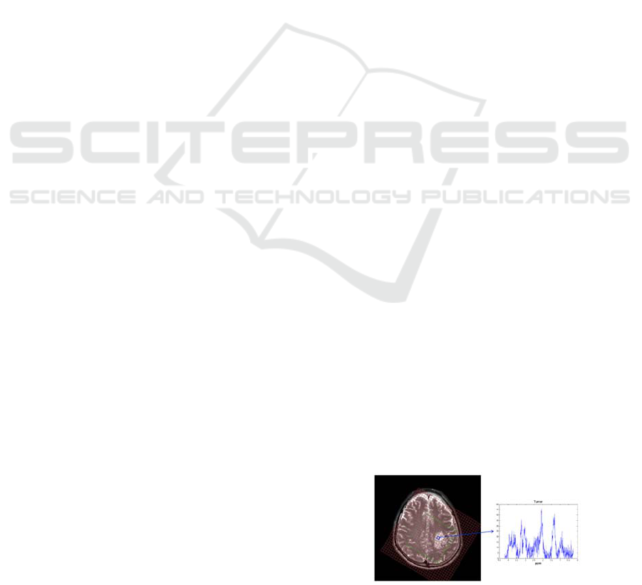
brain tumors; see Figure 1. Given an
mn×
matrix X
which represents the observed spectra from MRSI
data, each column containing a spectrum from one
voxel, previous studies (Su et al., 2008)
demonstrated that
X
can be approximately
described as a linear combination of constituent
specta of different tissue types. The model is
XWHN=+
(1)
W is a mr× matrix, with each column representing
a recovered spectrum for each tissue type. Each row
of the
rn
×
matrix H contains the linear
combination weights (interpreted here as abundances
or concentrations) of all constituent tissue spectra. N
stands for additive measurement noise.
Figure 1: Left: anatomic image of a glioma patient’s brain
overlaid with the MRSI grid. Right: the spectral profile
from the blue voxel from the tumor area.
Blind Source Separation (BSS) is one of the
main approaches to perform such factorization. One
of the algorithms, non-negative matrix factorization
(NMF) (Lee et al., 1999), has attracted much
212
Li Y., Sima D., Van Cauter S., Himmelreich U., Pi Y. and Van Huffel S..
SIMULATION STUDY OF TISSUE TYPE DIFFERENTIATION USING NON-NEGATIVE MATRIX FACTORIZATION.
DOI: 10.5220/0003734702120217
In Proceedings of the International Conference on Bio-inspired Systems and Signal Processing (BIOSIGNALS-2012), pages 212-217
ISBN: 978-989-8425-89-8
Copyright
c
2012 SCITEPRESS (Science and Technology Publications, Lda.)

attention in recent years because it does not require
the constituent spectra to be orthogonal or
independent. The mathematical formulation of the
basic NMF problem is
2
,
1
min ( , ) || ||
2
,, 0
F
WH
ij ij
fWH X WH
subject to ij W H
=−
∀≥
(2)
In this paper, we designed a simulation study
aiming to evaluate the accuracy of several popular
NMF implementations in solving the brain glioma
tissue type differentiation problem. The algorithms’
performance was investigated specifically in terms
of their accuracy to estimate tissue-specific spectra
and their spatial distribution.
2 NMF ALGORITHMS
In this section we describe several NMF algorithms
that will be compared in Section 4.
Multiplicative update method using Euclidean
distance measure (mu) (Lee et al., 2001):
This algorithm is used most commonly in
solving the NMF problem. It uses the Euclidean
distance as a measure to construct the cost
function
2
|| ||XWH−
. The cost function is
minimized using the update rule:
()
()
()
()
,,
T
kj
kj kj
T
kj
T
ik
ik ik
T
ik
WX
HH
WWH
XH
WW
WHH
ijk
←
←
∀
(3)
Alternating least squares (als) (Berry et al.,
2007): This algorithm alternately solves
unconstrained least squares subproblems for W
and H (see Eq. 4) and sets the negative elements
to zero.
2
2
argmin || ||
argmin || ||
F
F
WXWH
HXWH
←−
←−
(4)
Alternating non-negative least squares using
projected gradients (cjlin) (Lin, 2007): In this
implementation, non-negatively constrained least
squares subproblems are solved alternatively for
W and H using the projected gradient method.
Consider the following standard form of bound-
constrained optimization problems:
min ( )
: , 1,...,
n
xR
iii
fx
s
ubject to l x u i n
∈
≤≤ =
(5)
Projected gradient methods are iterative and
update the current solution
k
x
to the following
1k
x
+
by the rule:
1
[()]
kkkk
x
Px f x
α
+
=−∇
(6)
where
k
α
is the step size and
[]
i iii
ii ii
ii
x
if l x u
Px u if x u
lifxl
<<
⎧
⎪
=≥
⎨
⎪
≤
⎩
Hierarchical alternating least squares (hals)
(Cichocki et al., 2007; Cichocki et al., 2009):
hals
sequentially estimates one column of W and/or
one row of H while fixing all the other ones, that is
:
2
::0
2
0:
2
::0
2
0:
||||minarg
||||minarg
||||minarg
||||minarg
:
:
:
:
FkkkkH
FHk
FkkkkW
FWk
HWHWX
WHXH
HWHWX
WHXW
k
k
k
k
−−
=−←
−−
=−←
−−≥
≥
−−≥
≥
(7)
where W
:k
, W
-k
, H
k:
, H
-k
denote, respectively, the
kth column of W, the matrix W without the kth
column, the kth row of H, and the matrix H
without the kth row.
Accelerated multiplicative update method
(amu) and Accelerated HALS (ahals) (Gillis,
2011): These two more efficient methods are
developed based on the mu and hals methods.
Computational cost is reduced by updating W
several times before updating H (and vice versa),
instead of updating W and H alternately. An
inner loop stopping criterion is utilized for each
()l
W
, defined as the iterate after l updates of W
using Eq. 3 for amu or Eq. 7 for ahals (while H
is being kept fixed):
(1) () (1) (0)
|| || || ||
ll
F
F
WW WW
δ
+
−≤ −
(8)
where
δ
is a small constant, equal to 0.01 in the
implementation.
3 EXPERIMENT & RESULTS
3.1 Simulated Spatial Distribution
In order to construct a realistic MRSI grid
Containing spectra from normal tissue, as well as
SIMULATION STUDY OF TISSUE TYPE DIFFERENTIATION USING NON-NEGATIVE MATRIX
FACTORIZATION
213

tumor tissue and necrosis, we simulated an MRSI
grid in which these 3 tissue types are contained.
Table 1 shows the simulated distribution of brain
tissues. Each table cell represents a voxel. C, N, and
T denote respectively control tissue type (i.e.,
normal tissue), tumor tissue and necrotic tissue. In
the voxels at the interface between tissues, there is
usually a mixture of different tissue types.
Therefore, decimals are placed into the table to
represent concentration of mixed tissues. For
instance, 0.8C+0.2T denotes the tissue type in a
voxel composed of approximately 80% normal and
20% tumor tissue.
3.2 Simulated MRSI Signals
In our study, the simulated signals are linear
combinations of 9 metabolite profiles (two simulated
lipid profiles and seven metabolite profiles measured
in vitro), i.e., creatine (Cre), glutamate (Glu), myo-
inositol (Myo), phosphocholine (PCh), N-acetyl-
aspartate (NAA), alanine (Ala), lactate (Lac), lipid at
1.3ppm (Lip1), and lipid at 0.9ppm (Lip2). These
components are significant biomarkers for normal
brain tissue, tumor tissue, and necrosis tissue in
pathology (Howe et al., 2003). To choose proper
parameters for amplitude, damping, phase and
frequency for the simulated signals, we rely on a
parameter extraction procedure (Poullet et al., 2006).
In order to emulate the variability within an
MRSI grid, 4dB white Gaussian noise, which is in
agreement with our in vivo signals, is added to the
spectrum of each voxel.
The generated time domain signals, each having
2048 points, are Fourier transformed into the
frequency domain, then truncated to the frequency
range of interest, 0.25 – 4.2 ppm.
The simulated tissue-specific spectra with noise
are shown in the first row of Figure 2 (in blue) and
are compared with spectra from a clinical in vivo
case as shown in the second row of Figure 2. The
simulated pure spectra are in red.
3.3 Tissue Type Differentiation using
NMF Algorithms
Several NMF algorithms listed in section 2 are
applied to the simulated grid described in section 3.1;
see Table 1. The number of brain tissue types is set
to be 3, indicating normal tissue, tumor tissue and
necrotic tissue. The recovered constituent spectra
and their corresponding spatial distributions show
the variability of tissue type differentiation using
each of the described NMF algorithms; see Figure 3.
After scaling and normalization, we notice that
similar spectra with important peaks, which are
biomarkers for discrimination of different tissue
types (NAA, Cho, Lac/Lip), are obtained for each
tissue type with all methods. The corresponding
abundance maps clearly show the location of each
tissue type.
Table 1: Simulated tissue-specific spatial distribution. C denotes control tissue type, i.e., normal tissue. T denotes tumor
tissue. N denotes necrotic tissue.
C C C C C C C
0.8C
+0.2T
0.3C
+0.7T
T T
0.6T
+0.4N
T
C C C C C C C
0.8C
+0.2T
0.3C
+0.7T
T T
0.3T
+0.7N
0.5T
+0.5N
C C C C C C C
0.8C
+0.2T
0.3C
+0.7T
T
0.3T
+0.7N
0.2T
+0.8N
0.3T
+0.7N
C C C C C C C
0.8C
+0.2T
0.3C
+0.7T
T
0.1T
+0.9N
N
0.3T
+0.7N
C C C C C C C
0.8C
+0.2T
0.3C
+0.7T
T
0.1T
+0.9N
N
0.4T
+0.6N
C C C C C C C
0.8C
+0.2T
0.3C
+0.7T
0.5C
+0.5T
T
0.5T
+0.5N
0.5T
+0.5N
C C C C C C C C
0.8C
+0.2T
0.8C
+0.2T
0.5C
+0.5T
0.3C
+0.7T
0.5C
+0.5T
C C C C C C C C C C
0.8C
+0.2T
0.8C
+0.2T
0.8C
+0.2T
C C C C C C C C C C C C C
C C C C C C C C C C C C C
C C C C C C C C C C C C C
BIOSIGNALS 2012 - International Conference on Bio-inspired Systems and Signal Processing
214
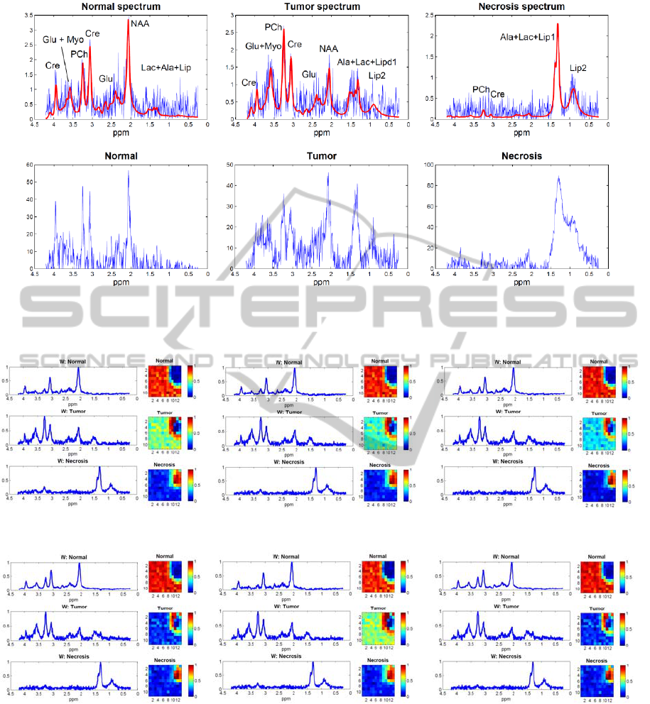
Figure 2: Spectra with SNR of 4dB from different voxels. The first row shows simulated spectra from normal tissue, tumor
tissue and necrotic tissue, respectively. Simulated noiseless spectra are shown with thick red lines. For comparison, the last
row contains in vivo spectra from the three different tissue types.
(a) (b) (c)
(d) (e) (f)
Figure 3: Simulation results of normalized recovered spectra (left column) and their corresponding spatial distribution (right
column) averaged over successful runs among 500 runs with different initializations using several NMF algorithms: (a) mu;
(b) cjlin; (c) als; (d) hals; (e) amu; (f) ahals. The color bars show scales for the distribution of concentration.
3.4 Validation of Spectral Separation
and Abundance Estimates
In order to evaluate the accuracy of the algorithms
listed in section 2, averaged results from 500 runs
(results with convergence problems were excluded,
i.e. 8 out of 500 runs for mu, 9 out of 500 runs for
als) for each algorithm were calculated, with
different starting values. For every run, all the
methods take the same initial value. Specifically,
SIMULATION STUDY OF TISSUE TYPE DIFFERENTIATION USING NON-NEGATIVE MATRIX
FACTORIZATION
215

correlation coefficients R between constituent
spectra estimated by NMF and simulated spectra are
computed. The closer R to 1, the better the similarity
between spectra generated using NMF and the
simulated spectra, thus the better the performance.
Furthermore, we compute the error rate of the
corresponding spatial distribution for each tissue
type:
2
2
()
100%
es
s
hh
ErrorRate
h
−
=⋅
∑
∑
(9)
where
e
h is the estimated abundance map from
NMF and
s
h
is the original distribution (see Table 1)
When the value of the error is lower, the accuracy of
the estimated spatial distribution is higher.
Algorithms were adjusted to make sure they all
detect convergence according to the same stopping
criterion, namely the condition that
(1) ()
|| ||
tt
WW
+
−
or
(1) ()
|| ||
tt
HH
+
− (i.e., the difference of recovered
sources or the recovered abundance maps in
subsequent iterations) drops below a certain
tolerance level, set to
4
10
−
for all the methods.
Results are shown in Figure 4. Overall, hals
gives the best result for all tissue types, especially
the error rate calculated by hals for tumor is
significantly lower than for other methods. Results
of ahals were also investigated but not shown here
since they are identical to hals.
(a) (b)
Figure 4: Accuracy evaluation. (a) correlation coefficient;
(b) error rate.
4 DISCUSSION & CONCLUSION
In this simulation study, we aimed at comparing the
performance of several NMF algorithms on spectra
with a high noise level. Spectral distortions due to,
e.g., magnetic field inhomogeneity and the chemical
shift displacement effect may lead to more signal
variability and to the violation of the model in Eq.1.
We chose not to include such non-linear factors of
variability in the simulations because those would
obscure the reasons for differences between
methods. Nevertheless, in vivo signals need to be
reprocessed and significantly distorted signals need
to be excluded before spectral separation using
NMF.
Among the tested NMF implementations, Lee
and Seung’s algorithm mu (Lee et al., 2001) was the
most commonly used one in the past. Comparisons
between various NMF algorithms have already been
presented in the literature (Kim et al., 2007). But
previous comparisons between algorithms were
mostly focused on evaluating computational
efficiency and divergence problems (Kim et al.,
2007; Cichocki et al., 2009), which are indicated by
the cost function
2
|| ||
F
XWH−
. However, the
accuracy of estimated tissue type profiles and the
corresponding spatial location is much more
important in the clinical diagnosis than
computational speed since the computing time of all
the methods is affordable for the dimensions of the
considered MRSI grids. Instead of evaluating the
results only visually, we follow (Croitor Sava et al.,
2010) who calculated correlation coefficients
between the obtained tissue sources and reference
tissue models. Our error rate is calculated between
the estimated spatial information and the simulated
spatial information. In this way, the accuracy of the
estimated spatial distribution of each tissue type can
be evaluated.
Overall, our results show that (a)hals gives the
best results in the simulation study, which confirms
the argumentation in (Gillis, 2011) that (a)hals has
remarkable performances. Especially the error for
tumor tissue shows a significant decrease compared
to all other methods. It demonstrates that the very
recent NMF algorithms hals and ahals can be
suitable for solving brain tissue type differentiation
problems using MRSI signals. In another study, we
further validate the feasibility of utilizing NMF
algorithms for brain tumor tissue differentiation
using in vivo MRSI signals.
ACKNOWLEDGEMENTS
This research was supported by Research Council
KUL: GOA MaNet, CoE EF/05/006 Optimization in
Engineering (OPTEC), PFV/10/002 (OPTEC), IDO
08/013 Autism, several PhD/postdoc & fellow grants;
Flemish Government: FWO: PhD/postdoc grants,
projects: FWO G.0302.07 (SVM), G.0341.07 (Data
fusion), G.0427.10N (Integrated EEG-fMRI),
G.0108.11 (Compressed Sensing) research
communities (ICCoS, ANMMM); IWT:
BIOSIGNALS 2012 - International Conference on Bio-inspired Systems and Signal Processing
216

TBM070713-Accelero, TBM070706-IOTA3,
TBM080658-MRI (EEG-fMRI), PhD Grants; IBBT
Belgian Federal Science Policy Office: IUAP P6/04
(DYSCO, `Dynamical systems, control and
optimization', 2007-2011); ESA AO-PGPF-
01, PRODEX (CardioControl) C4000103224;
EU: RECAP 209G within INTERREG IVB NWE
programme, EU HIP Trial FP7-HEALTH/ 2007-
2013 (n° 260777) (Neuromath (COST-BM0601):
BIR&D Smart Care. Li thank the China Scholarship
Council.
REFERENCES
Berry M, Browne M, Langville A, Pauca V, and
Plemmons R, 2007. Algorithms and applications for
approximate non-negative matrix factorization.
Comput Stat Data Anal,52:155-173.
Brown T, Kincaid B, Ugurbil K, 1982. NMR chemical
shift imaging in three dimensions. PNAS, 79(11):
3523-3526.
Cichocki A, Zdunek R, Amari S, 2007. Hierarchical ALS
algorithms for nonnegative matrix and 3D tensor
factorization. Lect Notes Comput Sci, 4666:169-176.
Cichocki A, Phan AH, 2009. Fast local algorithms for
large scale Nonegative Matrix and Tensor
Factorizations. IEICE Trans Fund Electron Comm
Comput Sci, 3:708-721.
Croitor Sava AR, Sima DM, Martinez-Bisbal MC, Celda
B, Van Huffel S, 2010. Non-negative Blind Source
Separation Techniques for Tumor Tissue Typing
Using HR-MAS signals. In Proceedings of the 32nd
Annual International Conference of the IEEE EMBS,
Buenos Aires, Argentina.
Gillis N, 2011. Nonnegative matrix factorization
complexity, algorithms and applications. PhD Thesis,
Louvan-La-Neuve, Belgium.
Gonzalez EF, Zhang Y, 2005. Accelerating the Lee-Seung
algorithm for non-negative matrix factorization. Tech
Report, Rice University.
Grippo L, Sciandrone M, 2000. On the convergence of the
block nonlinear Gauss-Seidel method under convex
constraints. Oper Res Letter, 26:127-136.
Howe FA, Barton SJ, Cudlip SA, Stubbs M, Saunders DE,
Murphy JR, Opstad KS, Doyle VL, McLean MA, Bell
BA, Griffiths JR, 2003. Metabolic profiles of human
brain tumours using quantitative in vivo 1H magnetic
resonance spectroscopy. Magn Res Med,49:223-232.
Jolliffe IT. Principal Component Analysis. Second edition,
New York: Springer-Verlag 2002. 487 p.
Kim D, Sra S., Dhillon IS, 2007. Fast Newton-type
Methods for the Least Squares Nonnegative Batrix
Approximation Problem. In Proceedings of the 2007
SIAM International Conference on Data Mining
(ICDM), Pisa, Italy.
Ladroue C, Howe FA, Griffiths JR, Tate AR, 2003.
Independent component analysis for automated
decomposition of in vivo magnetic resonance spectra.
Magn Reson Med, 50:697-703.
Lee DD, Seung HS, 1999. Learning the parts of objects by
non-negative matrix factorization. Nature, 401:788-
791.
Lee DD, Seung HS, 2001. Algorithms for Non-negative
Matrix Factorization, Advances in Neural Information
Processing Systems, 13:556-562.
Lin CJ, 2007. Projected Gradient Methods for
Nonnegative Matix Factorization, Neural Comput,
19:2756-2779.
Poullet JB, Sima DM, Simonetti AW, De Neuter B,
Vanhamme L, Lemmerling P, Van Huffel S, 2006. An
automated quantitation of short echo time MRS
spectra in an open source software environment:
AQSES. NMR Biomed, 20: 493-504.
Stoyanova R, Brown TR, 2001. NMR spectral quantitation
by principal component analysis. NMR Biomed,
14:260-264.
Su Y, Thakur SB., Karimi S, Du S, Sajda P, Huang W,
Parra LC, 2008. Spectrum separation resolves partial-
volume effect of MRSI as demonstrated on brain
tumor scans. NMR Biomed
, 21:1030-1042.
Szabo de Edelenyi F, Simonetti AW, Postma G, Huo R,
Buydens LMC, 2005. Application of independent
component analysis to 1H MR spectroscopic imaging
exams of brain tumours. Anal. Chim. Acta, 544:36-46.
SIMULATION STUDY OF TISSUE TYPE DIFFERENTIATION USING NON-NEGATIVE MATRIX
FACTORIZATION
217
