
SIFT-BASED CAMERA LOCALIZATION USING REFERENCE
OBJECTS FOR APPLICATION IN MULTI-CAMERA
ENVIRONMENTS AND ROBOTICS
Hanno Jaspers
1
, Boris Schauerte
2
and Gernot A. Fink
1
1
Department of Computer Science, TU Dortmund University, 44221 Dortmund, Germany
2
Institute of Anthropomatics, Karlsruhe Institute of Technology, 76131 Karlsruhe, Germany
Keywords:
Camera pose estimation, Relative pose, Camera calibration, Scale Ambiguity, Reference object, Local
features, SIFT, Multi-camera environment, Smart room, Robot localization.
Abstract:
In this contribution, we present a unified approach to improve the localization and the perception of a robot
in a new environment by using already installed cameras. Using our approach we are able to localize arbi-
trary cameras in multi-camera environments while automatically extending the camera network in an online,
unattended, real-time way. This way, all cameras can be used to improve the perception of the scene, and ad-
ditional cameras can be added in real-time, e.g., to remove blind spots. To this end, we use the Scale-invariant
feature transform (SIFT) and at least one arbitrary known-size reference object to enable camera localization.
Then we apply non-linear optimization of the relative pose estimate and we use it to iteratively calibrate the
camera network as well as to localize arbitrary cameras, e.g. of mobile phones or robots, inside a multi-camera
environment. We performed an evaluation on synthetic as well as real data to demonstrate the applicability of
the proposed approach.
1 INTRODUCTION
In recent years smart rooms have attracted an increas-
ing interest, e.g., to improve the productivity in of-
fice environments and assist the personnel in crisis
response centers. For this purpose, the identities of
the persons in the room have to be determined (see
(Salah et al., 2008)) as well as the audio-visual focus
of attention has to be estimated (see (Voit and Stiefel-
hagen, 2010; Schauerte et al., 2009)), e.g. to present
personalized information on the display a person is
currently looking at. However, these applications rely
on the fusion of information that is provided by a set
of sensors, most importantly microphones and camera
arrays. In order to fuse the information from different
sensors in the environment it is necessary to deter-
mine their extrinsic parameters in a common coordi-
nate frame. In the following, we focus on cameras as
sensors and in this domain offline calibration meth-
ods are applied most commonly (see, e.g., (Br
¨
uck-
ner and Denzler, 2010; Aslan et al., 2008; Xiong and
Quek, 2005; Rodehorst et al., 2008)). Unfortunately,
these methods usually require a time-consuming man-
ual procedure and need to be repeated if a new camera
is added or a camera is relocated.
In this contribution, we analyze how we can use
the views of the already calibrated cameras in an en-
vironment to localize a new camera and thus enable
subsequent sensor fusion. This, for example, can be
used to enable easily extensible camera networks, al-
low the seamless integration of the sensor information
of mobile robotic agents , and allow mobile robotic
agents to use the information of the sensors that are
installed in the environment to enhance their percep-
tion capabilities. With the proposed approach, we are
able to determine the absolute pose of a new cam-
era in the global coordinate system given only one
known camera and an arbitrary reference object. Al-
though our focus on a single known camera may limit
the achievable results in scenarios with a huge amount
of cameras with widely overlapping views, we chose
this focus, because it enables us to integrate cameras
that only view parts of the scene that are recorded by
only one other camera. This is especially important,
if the viewpoints of the cameras are very different or
only few cameras are used, which – according to our
experience – seems to be more realistic in most ap-
plication areas. However, our method can naturally
be extended to situations with multiple views. To this
end, we calculate the poses for all plausible camera
330
Jaspers H., Schauerte B. and Fink G. (2012).
SIFT-BASED CAMERA LOCALIZATION USING REFERENCE OBJECTS FOR APPLICATION IN MULTI-CAMERA ENVIRONMENTS AND ROBOTICS.
In Proceedings of the 1st International Conference on Pattern Recognition Applications and Methods, pages 330-336
DOI: 10.5220/0003735103300336
Copyright
c
SciTePress

pairs and subsequently aggregate the pairwise local-
ization results. In contrast to most previous work, we
do not rely on special calibration patterns or devices
and use arbitrary reference objects instead
1
. To this
end, only a very small amount of user interaction is re-
quired to build an appropriate database of known ob-
jects. The necessary information about the reference
objects might be automatically collected from the in-
ternet, or in the domain of cognitive robots, directly
obtained by actively exploring potential objects. Once
the information is available, cameras can be localized
completely automatic at any time.
2 RELATED WORK
The research area of camera calibration, of which
camera pose estimation is an important aspect, is
a well known and researched topic and accordingly
many different approaches have been proposed (see,
e.g., (Br
¨
uckner and Denzler, 2010; Aslan et al., 2008;
Frank-Bolton et al., 2008; Xiong and Quek, 2005;
Rodehorst et al., 2008)).
In order to calculate the relative pose, the funda-
mental matrix has to be computed. The normalized
and the standard 8-point algorithm, variants of the
7-point algorithm (Hartley and Zisserman, 2004), as
well as a 6-point and 5-point algorithm were com-
pared (Stew
´
enius et al., 2006; Nist
´
er, 2004). The
normalized 8-point algorithm performed considerably
better than the non-normalized version and its use
was recommended when no prior knowledge about
the camera motion, i.e. sideways or forward mo-
tion, is available. The 5-point algorithm achieved bet-
ter results in most cases, as confirmed in (Rodehorst
et al., 2008), but it had problems with forward motion,
where the results were worse. We used the 8-point al-
gorithm in our approach because of its overall good
results.
For finding point correspondences, we rely on
the matching of SIFT features, proposed by Lowe in
(Lowe, 1999; Lowe, 2004). In the context of relative
pose estimation and scene reconstruction, SIFT has
been used before in (Liu and Hubbold, 2006; Snavely
et al., 2008).
In previous work, (Xiong and Quek, 2005) de-
scribed a system to calibrate the intrinsic and extrin-
sic parameters of camera networks in meeting rooms.
They used a box with dots and other markers to cali-
brate the cameras. This resulted in a good accuracy of
less than 1cm for the camera positions of most cam-
eras. However, a lot of user interaction is required
1
However, we could – of course – use existing calibra-
tion patterns and objects as reference objects as well.
to perform the calibration: Camera pairs were chosen
manually and the calibration box had to be placed for
each camera pair specifically.
(Svoboda et al., 2005) proposed a technique with
less user interaction for the calibration of a multi-
camera environment. Instead of using dedicated cal-
ibration objects or markers, they used a bright spot
as the calibration feature, generated by a laser pointer
with a small diffusing piece of plastic attached to it.
Their algorithm can be used to fully calibrate the cam-
era network, the only user interaction is waving the
laser pointer through the working volume.
Aslan et al. pursued a similar approach to auto-
matically calibrate the extrinsic parameters of multi-
ple cameras (Aslan et al., 2008). Instead of a bright
spot, they detected people walking through the room
and used a point on top of every person’s head as cal-
ibration feature. The relative pose is estimated for ev-
ery camera pair, and with this, the complete camera
network is built up using a global error minimization
technique. The precision has been evaluated in differ-
ent indoor scenarios, arriving at a projection error of
less than 6px and a triangulation error of markers in
the scene of about 5cm. The positions of the camera
centers have not been compared to their ground truth.
Recently, Br
¨
uckner and Denzler proposed an ac-
tive calibration technique for multi-camera systems
(Br
¨
uckner and Denzler, 2010). They use the rotat-
ing and zooming capabilities of pan-tilt-zoom (PTZ)
cameras to optimize the relative poses between each
camera pair. The scaling factors in camera triangles
are estimated with two of the three relative poses. In
contrast to our approach no reference object is re-
quired, but the types of cameras that can be used are
limited to PTZ cameras. Our system does not put any
limitations on the types of cameras, allowing, for ex-
ample, a combination of fixed PTZ cameras, cameras
mounted on robotic platforms and even smartphone
cameras. Furthermore, more than two cameras are
needed, whereas our approach allows to estimate the
absolute pose of only two cameras.
Similar techniques as those used for the calibra-
tion of multi-camera environments can be applied to
other applications, such as robot indoor localization.
In (Frank-Bolton et al., 2008), a system to localize
and track a robot based on a set of known views was
proposed. First, a set of views of the scene, an in-
door environment, was recorded with the robot for
specific positions and different orientations. The posi-
tions were chosen on a grid, roughly 90cm apart. The
environment was surrounded by project posters to fa-
cilitate the search for image correspondences. Frank-
Bolton et al. come to the conclusion, that epipolar
geometry in conjunction with the normalized 8-point
SIFT-BASED CAMERA LOCALIZATION USING REFERENCE OBJECTS FOR APPLICATION IN
MULTI-CAMERA ENVIRONMENTS AND ROBOTICS
331
Estimation of Relative Pose
using Epipolar Geometry
Relative Pose Optimization
of Reprojection Error
Computation of Scale
via Homography
Reference Object
Absolute Pose
Image 1 Image 2
Intrinsic
Parameters
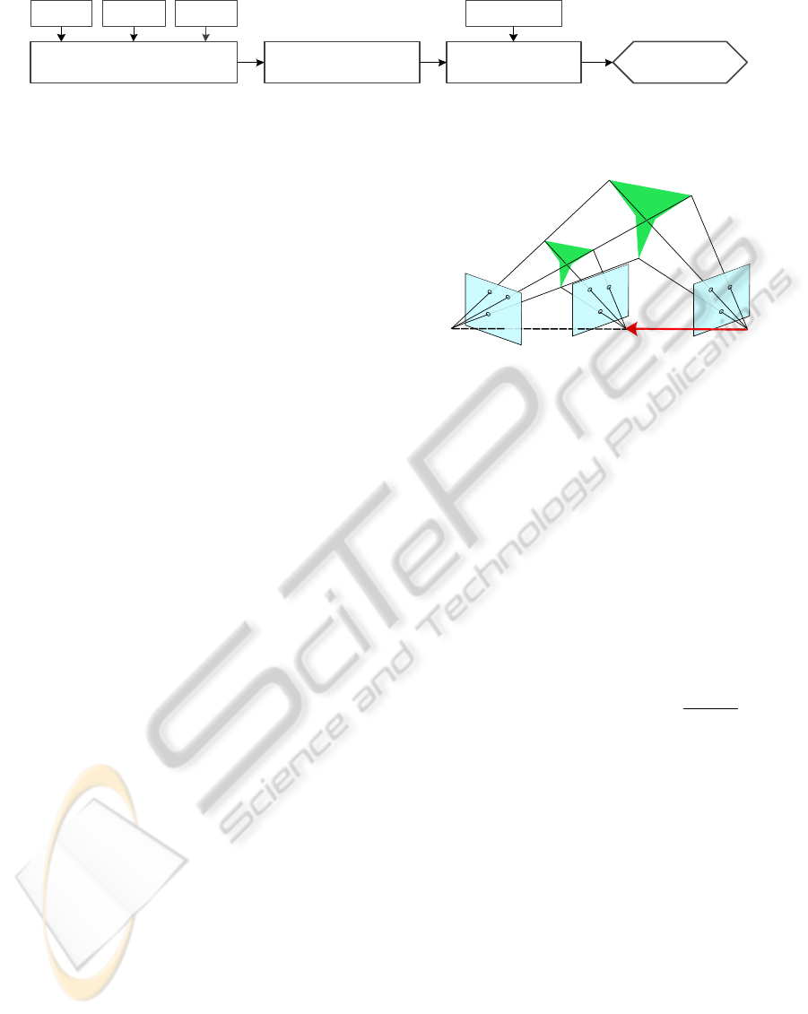
Figure 1: This overview of our approach shows the three main steps to calculate the absolute pose of a camera. At first the
relative pose is estimated using epipolar geometry. Afterwards, the relative pose is optimized and then scaled with a scaling
factor retrieved from a known reference object, giving the absolute pose of the second camera in relation to the first camera.
algorithm is too sensitive to ensure a robust and ac-
curate pose estimation. Instead, they use a technique
called quality threshold clustering, which resulted in
an average position error of 46cm and a mean orienta-
tion error of 9
◦
. Our results (see section 4) lead to the
assumption, that a more precise localization can be
achieved with our approach, using the project posters
as reference objects.
3 POSE ESTIMATION
Our sytem that computes the global pose of a camera
in relation to a known camera consists of three main
steps (see Fig. 1). In the first step, the relative pose of
the camera is calculated. This requires the detection
of point correspondences between the two considered
images. To this end, SIFT features (Lowe, 2004) are
computed and matched. This step may introduce out-
liers, i.e. correspondences of image points that are
not projections of the same scene point. If they are
not robustly eliminated, errors in the estimated pose
will occur. In the second step we optimize the esti-
mated relative pose in order to minimize the influence
of noise and achieve better results. Finally, the global
scaling of the relative pose is calculated in the third
step. This step is based on the detection of at least
one reference object of known size within the scene.
3.1 Relative Pose
The relative pose of the second camera is calculated
using epipolar geometry. For this, the fundamental
matrix F is calculated with the normalized 8-point al-
gorithm in conjunction with RANSAC, to eliminate
outliers from the point correspondences (Hartley and
Zisserman, 2004). Using the fundamental matrix the
scene can be reconstructed up to a projective ambigu-
ity. We assume calibrated cameras with the intrinsic
calibration matrices K
1
and K
2
. Accordingly, the re-
construction can be performed up to a scale ambigu-
ity, as illustrated in Fig. 2. As a result of the unknown
scale, the translation vector t is normalized to ktk = 1.
The essential matrix E, a special case of the fun-
damental matrix for normalized image coordinates, is
Figure 2: Visualization of the scale ambiguity. The second
camera can ”slide” along the baseline between the cameras
(i.e. different scaling of the relative position), without af-
fecting the point correspondences.
obtained as
E = K
2
T
F K
1
. (1)
The defining property of the essential matrix is that
two of its singular values are equal and the third one
zero. Due to the presence of noise that is introduced
through small errors in the camera calibration pro-
cess and the estimation of the fundamental matrix,
this property has to be enforced. Thus, let
E = U diag(σ
1
, σ
2
, σ
3
) V
T
, with σ
1
≥ σ
2
≥ σ
3
(2)
be the SVD of E. The essential matrix
e
E, which min-
imizes the Frobenius norm kE −
e
Ek, is calculated as
e
E = U diag(σ, σ, 0) V
T
, with σ =
σ
1
+ σ
2
2
. (3)
The essential matrix can be decomposed into four
possible solutions for the pose (t, R) of the second
camera, with translation t and rotation R. There’s
only one solution for which the reconstructed 3D-
points are in front of the image planes of both cam-
eras. This constraint is termed cheirality constraint.
In ideal circumstances it would suffice to reconstruct
one point from a point correspondence pair and to test
whether it satisfies the cheirality constraint. But since
outliers can’t be ruled out a voting mechanism has to
be put in place to determine the correct solution: Each
reconstructed point ”votes” for the solution, that sat-
isfies its cheirality constraint. The solution with the
highest number of votes is chosen as the correct solu-
tion.
3.2 Pose Optimization
Figure 3(b) shows the reconstruction of a scene that
ICPRAM 2012 - International Conference on Pattern Recognition Applications and Methods
332
−150 −100 −50 0 50 100 150
0
50
100
150
200
250
300
x [cm]
y [cm]
(a)
−150 −100 −50 0 50 100 150
0
50
100
150
200
250
300
x [cm]
y [cm]
(b)
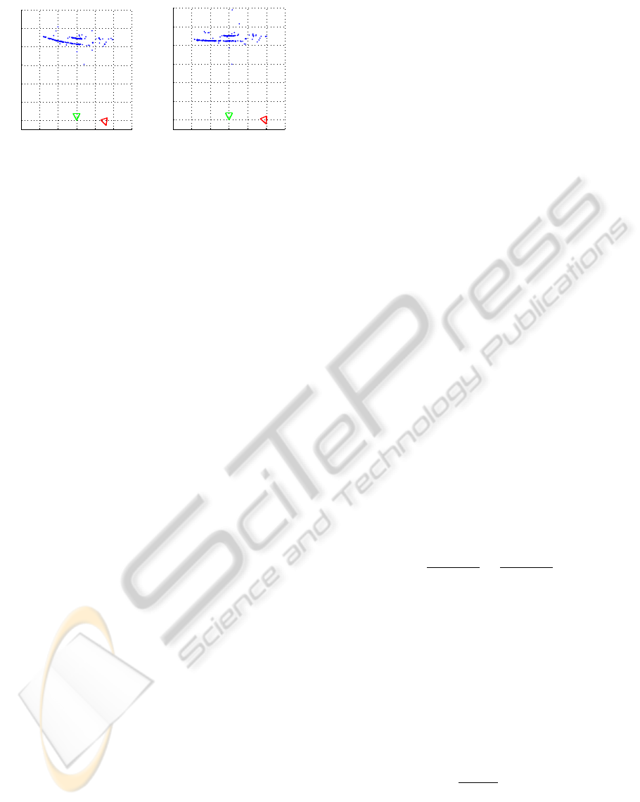
Figure 3: The relative pose of the red camera is estimated
(a) using only epipolar geometry, and (b) with additional
nonlinear optimization. With optimization, most of the re-
constructed points (blue) are parallel to the x-axis, which
complies with the ground truth.
was obtained using the relative pose as described
above. The camera was oriented towards a flat wall.
However, the reconstructed points lay on a curved
surface. This indicates small errors in the obtained
pose. To improve the relative pose, a nonlinear,
Trust-Region-Reflective optimization step (Coleman
and Li, 1996) has been introduced that minimizes
the reprojection error. In contrast to Levenberg-
Marquardt optimization (Levenberg, 1944; Mar-
quardt, 1963), Trust-Region-Reflective optimization
can handle bound constraints on the optimization
space.
A pose normally has six degrees of freedom
(DOF), three for the translation and three for the rota-
tion. As a result of the scale ambiguity, this is reduced
to five DOF for the relative pose.
Because of the normalization ktk = 1, all possible
solutions for t are on the unit sphere around the first
camera. Hence, t can be expressed in spherical coor-
dinates (θ, φ). Together with the rotation angles r
x
, r
y
and r
z
, the optimization space is (θ, φ, r
x
, r
y
, r
z
). As
the optimization step only finds a local minimum of
the reprojection error, a good initial guess is impor-
tant in order to find the global minimum. Thus, the
starting point for the optimization task is the relative
pose as computed before.
Depending on the application, further constraints
may exist, which reduce the dimension of the opti-
mization space. For example, in a room equipped
with PTZ cameras, r
z
(roll) can be fixed to 0.
3.3 Solving the Scale Ambiguity
When given only two views of a scene, the solution
for the scale ambiguity problem requires more infor-
mation on the scene itself or the objects located in it.
Our approach uses the knowledge of reference objects
that have been detected, using SIFT, in both views.
The best results can be obtained with planar objects,
such as posters or pictures. Nevertheless, non-planar
objects are also possible as reference objects, but re-
quire certain restrictions or more complex processing
of the local features to achieve similar results.
The reference objects are detected by matching
an image of each reference object with both views
and calculating the projective transformations of the
objects. The matching is done with SIFT features.
This is an advantage since the SIFT features calcu-
lated for the estimation of the relative pose can be
reused. The projective transformations are homogra-
phies between the the reference objects and their oc-
curances in the two views. A homography is a pro-
jective transformation that maps points on one plane
to another plane (which is also the reason why pla-
nar reference objects yield the best results). It is for-
malized by a 3 × 3 matrix H, called the homography
matrix. An algorithm to compute the homography
is the direct-linear-transformation algorithm (Hartley
and Zisserman, 2004, p. 88), which can be combined
with RANSAC to ensure robustness against outliers.
Let H = [h
1
, h
2
, h
3
] be the homography matrix be-
tween the image of the reference object and one of
the views and K the intrinsic calibration matrix of the
camera. According to (Zhang, 2000) the extrinsic pa-
rameters [R|t] of the camera image in relation to the
reference object can be computed as
r
1
= λK
−1
h
1
, (4)
r
2
= λK
−1
h
2
, (5)
r
3
= r
1
× r
2
, (6)
t = λK
−1
h
3
, (7)
with
λ =
1
k
K
−1
h
1
k
=
1
k
K
−1
h
2
k
(8)
and the rotation matrix R = [r
1
, r
2
, r
3
].
The distance of the reference object (more exactly
the origin of the reference object’s image) to the cam-
era center is given by ktk. If the size of the object
is known in the units of the world coordinate system
(e.g. mm, as used in the following), then t can also
be expressed in this unit. Let d
px
be the size vector
(width and height) of the reference object’s image in
pixels, and d
mm
the size vector in millimeters. Thus,
the translation vector t scaled to millimeters is then
given as
ˆ
t =
k
d
mm
k
k
d
px
k
· t . (9)
Let x be the origin of the reference object’s image
in the scene. It can be reconstructed with the estimate
of the relative pose of the second camera as computed
previously. Thus, relating the translation vectors of
the reference object
ˆ
t
1
and
ˆ
t
2
to the distances between
SIFT-BASED CAMERA LOCALIZATION USING REFERENCE OBJECTS FOR APPLICATION IN
MULTI-CAMERA ENVIRONMENTS AND ROBOTICS
333
x and the camera centers c
1
and c
2
provides us with
two scaling factors:
s
1
=
ˆ
t
1
k
x − c
1
k
and s
2
=
ˆ
t
2
k
x − c
2
k
. (10)
These scaling factors are, in theory, equal, but usu-
ally differ slightly when estimated on real data. There
are two possibilities to use these factors to correctly
scale the yet unscaled position of the second camera:
ˆ
c
2a
=
1
2
(s
1
+ s
2
) · c
2
, and (11)
ˆ
c
2b
= s
1
(x − c
1
) + s
2
(x − c
2
) . (12)
The first possibility is straightforward and applies the
average scaling factor directly to the relative position
of the second camera. The second possibility applies
the scaling factors to the vectors between the camera
centers and the reference object. This has proven to
work better in scenes in which the reference object is
reliably and precisely detected, giving very accurate
scaling factors. In contrast, Eq. 11 achieves good
results for scenes in which the relative pose is very
precise, while the scaling factors are prone to noise,
which may occur with small reference objects.
4 EVALUATION
The evaluation of our system is divided into two parts,
synthetic and real benchmarks. The synthetic tests
evaluate the single components of our system, the es-
timation of the relative pose and the calculation of the
scale. To test our algorithm on real data, we used
the data sets presented in (Strecha et al., 2008) and
images recorded by ourselves in a smart room at our
university.
4.1 Synthetic Data
At first, we evaluated the relative pose estimation al-
gorithm to determine the influence of the optimiza-
tion on the result. For this purpose, we generated
200 random 3D points in a box of side length 2, cen-
tered at (0 0 3)
T
. We then projected these points on
two virtual cameras with intrinsic calibration matri-
ces K = I. The second camera was positioned ran-
domly on the unit sphere. For each position, the pose
was estimated 1000 times. We set the threshold of
RANSAC to 1000 iterations. To test the influence of
noise, we introduced white Gaussian noise of a certain
signal-to-noise ratio to the projected points. More de-
scriptively, on a 640 × 480px picture, a noise level of
50dB would be equivalent to a standard deviation of
about 1.4px, 30dB to 14px and 20dB to 43px. Out-
liers were inserted by selecting a certain percentage
of points and assigning them to other points.
The performance for different percentages of out-
liers is unaffected by the optimization. This is due to
the fact, that outliers are removed by RANSAC when
calculating fundamental matrix. The optimization af-
terwards does not affect the point correspondences.
We obtain very robust results up to a outlier percent-
age of 60%, with a translation error of less than 3
◦
and a rotation error of less than 1
◦
.
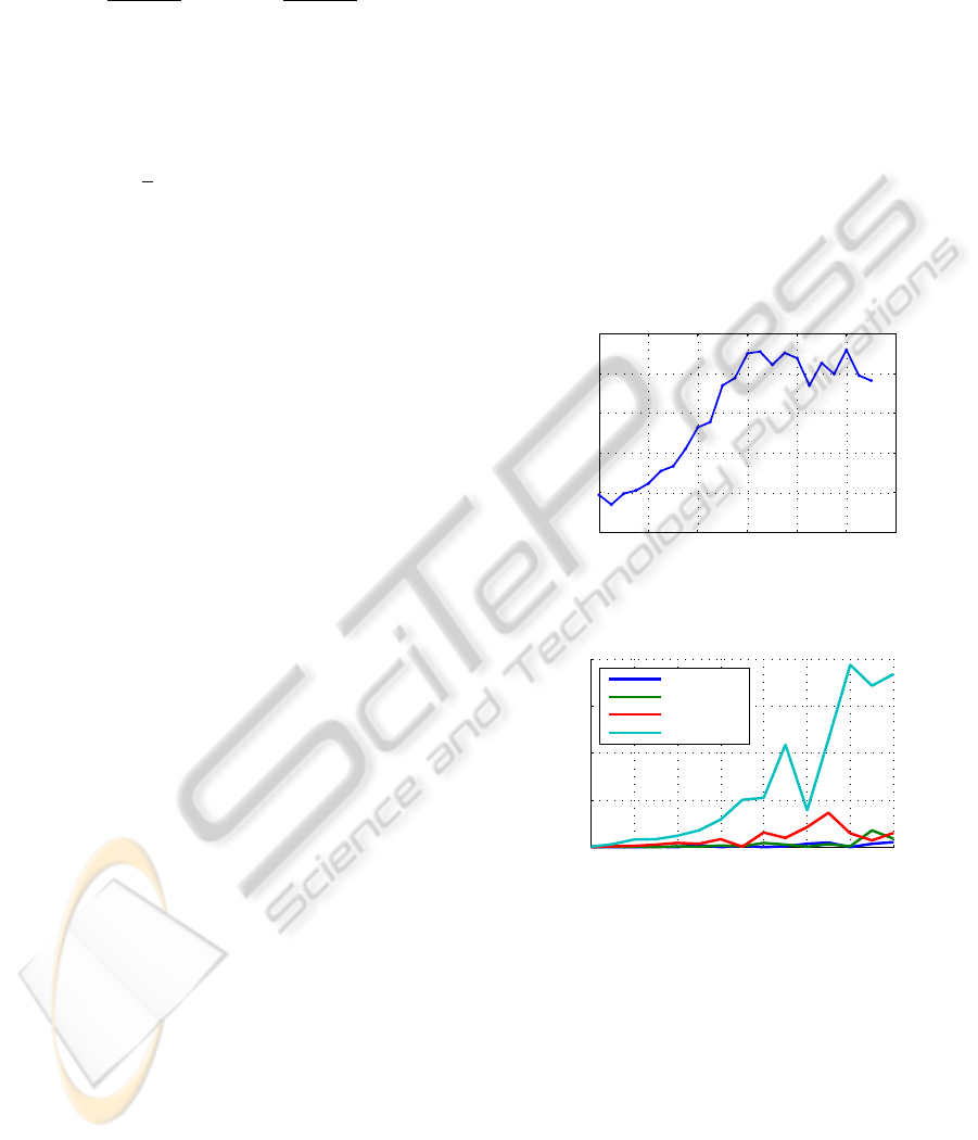
Figure 4 shows the improvement brought by the
optimization of the relative pose in the presence of
noise. The translation error is reduced by 31.6% for
noise levels starting at 25dB. The rotation error is
largely unaffected by the optimization.
0 10 20 30 40 50 60
−10
0
10
20
30
40
noise level [dB]
mean error improvement [%]
Figure 4: For noise levels starting at 25dB, the optimization
reduces the translation error by an average of 31%.
100 150 200 250 300 350 400 450
0
5
10
15
20
Distance to camera center [cm]
Error of computed distance [cm]
0° Rotation
15° Rotation
30° Rotation
45° Rotation
Figure 5: The graph shows the error of the calculated dis-
tance of a square reference object for different rotations.
To test, how accurate the distance of a reference
object can be estimated, a square reference object
with side lengths of 50cm was rotated around its y-
axis and positioned on different distances along the
z-axis. For every position and rotation an image was
created with a virtual camera with a focal length of
2000 and principal point [1000, 1000]
T
. The reference
object’s distance was retrieved as described in section
3.3, including its detection using SIFT and RANSAC-
based homography estimation. Each calculation was
repeated 100 times. The results, illustrated in Fig. 5,
show that the distance can be robustly computed for
ICPRAM 2012 - International Conference on Pattern Recognition Applications and Methods
334

all positions and rotations up to 30
◦
. The error is less
than 4cm and for most measurements less than 2cm.
Without rotation, the error is never above 1cm. For a
rotation of 45
◦
, the error increases to about 20cm at a
distance of 4m to 4.5m. This is still less than 5% of
the distance of the reference object.
4.2 Real Data
Furthermore, we evaluated our proposed approach
on different real data sets. The first tests use the
Herz-Jesu-P8 and fountain-P11 data sets (see (Strecha
et al., 2008)). We chose these data sets, because they
contain images with a high resolution and are well
annotated. We generated reference objects for both
data sets by cropping parts of the images, that showed
walls which were visible in most pictures. We re-
duced the data sets to those images, in which the ref-
erence object could be detected. The camera poses
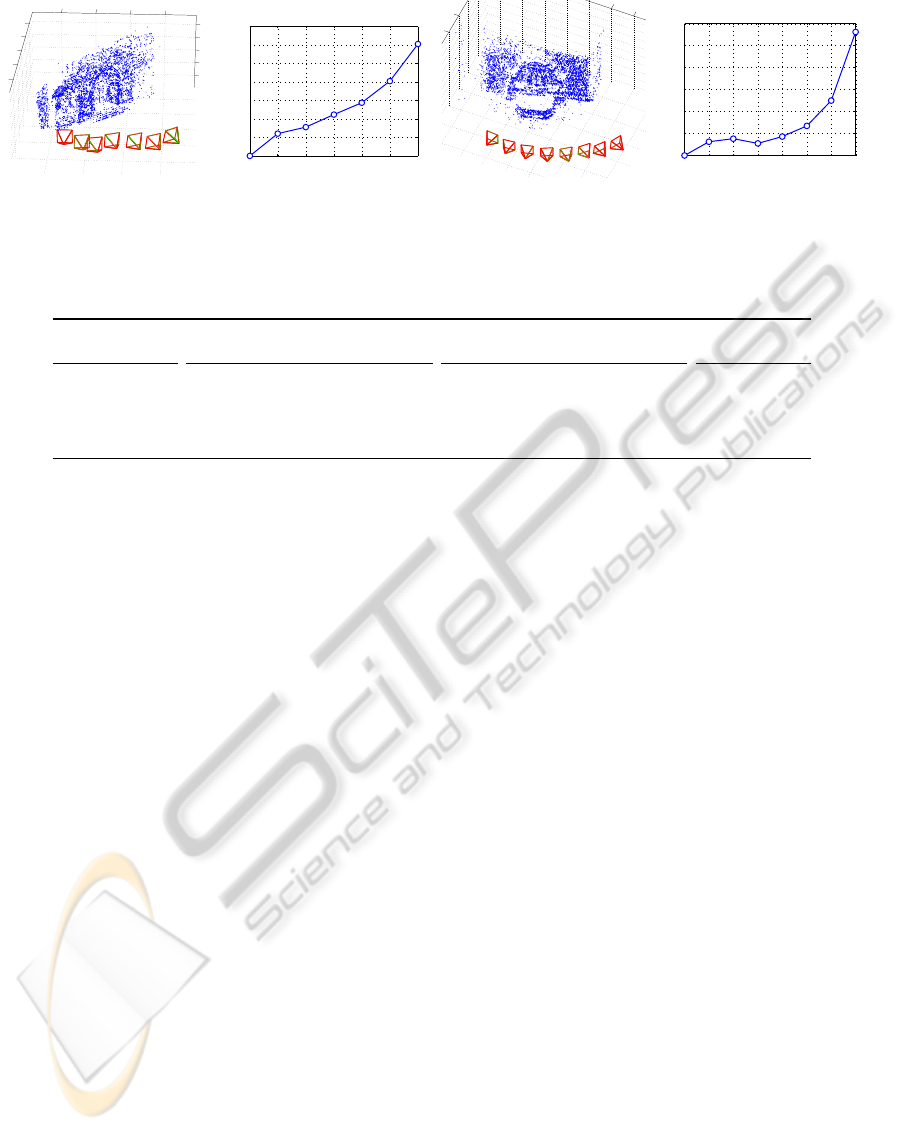
were calculated iteratively. Figure 6 shows the recon-
struction results and position errors for both data sets.
Since the camera poses are iteratively estimated,
small errors are propagated and increase in the pro-
cess of the computation. Still, the results are very
accurate and the errors are in the range of centime-
ters. Over a total distance of 15.5m in data set Herz-
Jesu-P8, the error of the last camera is only 12cm, or
0.77%. The distance between the first and last camera
in fountain-P11 is 11m, yet the position error is a mere
6cm, or 0.55%. The data sets have certain character-
istics that help attaining such a high precision: high
resolution, small baselines between the cameras and
highly textured scenes that produce well distributed
point correspondences.
These characteristics are less present in the data
recorded in our smart environment, a room of roughly
25m
2
. It has several microphone arrays, computer
controlled lighting and, most importantly for our case,
four ceiling-mounted PTZ cameras with a resolution
of 752 × 596 pixels. The position and rotation of the
PTZ cameras are known. Pictures were taken with a
similar PTZ camera on a tripod at 23 different posi-
tions in the room. The positions were measured by
hand in the environment’s coordinate frame to obtain
a ground truth. For each position, the absolute cam-
era pose was calculated several times using one of the
known cameras. The results with the lowest repro-
jection error for every image were selected and aggre-
gated by using the mean and the median of the coor-
dinates and then compared to the ground truth. Three
posters, two of size 118.9 × 84.1cm and one of size
60 × 91cm, were chosen as reference objects. Table 1
shows the attained results.
We arrive at a mean position error of 41.30cm for
the mean position and 39.50cm for the median posi-
tion. Compared to the much lower median position er-
ror of 25.24cm, and 21.64cm respectively, we see that
the camera was very poorly localized for several mea-
surement points, with an error of over 2m for cam-
era position 3 and about 1m for positions 16 and 17.
The poses for other positions were very close to the
ground truth, often with an error of less than 16cm.
There are different reasons for the high errors in
the detected poses for the images in our smart room.
Most importantly, the cameras provide noisy images
without much detail and fail to record fine structures.
Furthermore, the environment itself does not contain
much details, making it hard to find reliable point cor-
respondences. This is made even more difficult by the
the low number of cameras and big viewpoint changes
between the cameras. As a consequence, point cor-
respondences were often found mostly between the
projections of the reference objects and for this rea-
son only locally distributed in the images. Although
the error seems relatively large on the first sight –
especially when compared to the results achieved on
Herz-Jesu-P8 and fountain-P11 –, we consider a me-
dian error of 21.64cm an acceptable result due to the
difficulty of the environment. Furthermore, we have
to consider the possible influence of minor ground
truth measurement errors that were, for example, in-
troduced by the unknown exact location of the focal
point within the PTZ camera casing.
5 CONCLUSIONS
We proposed a new approach to compute the global
scale between two views given a known reference ob-
ject. To this end, we first calculate the relative pose
with established methods of epipolar geometry. We
then reduce the reprojection error of the pose with a
nonlinear optimization step, significantly improving
the result. Afterwards, the overall scale of the scene
is reliably estimated by detecting a known reference
object in both camera views. Through different tests,
our system has proven to very precisely compute ab-
solute poses. In two data sets with small distances
between camera images, we achieved an absolute er-
ror for the iterative pose estimation of less than 1%.
The global localization of cameras in our conference
room was less accurate, hindered by low resolution
cameras, plain walls without much detail and wide
baselines. However, we still achieved an accuracy of
about 20cm for most camera pairs, making our system
a useful and convenient technique for the extrinisc
calibration of multiple cameras.
SIFT-BASED CAMERA LOCALIZATION USING REFERENCE OBJECTS FOR APPLICATION IN
MULTI-CAMERA ENVIRONMENTS AND ROBOTICS
335
−5
0
5
10
15
−15
−10
−5
0
−8
−6
−4
−2
0
7
6
5
4
3
2
1
(a)
1 2 3 4 5 6 7
0
2
4
6
8
10
12
14
Camera index
Error [cm]
Herz−Jesu−P8: Position error, iterative calculation
(b)
−14
−12
−10
−10
−8
1
2
3
4
5
6
7
8
y
(c)
1 2 3 4 5 6 7 8
0
1
2
3
4
5
6
Camera index
Error [cm]
fountain−P11: Position error, iterative calculation
(d)
Figure 6: The scene reconstruction and position error of data sets Herz-Jesu-P8 (a-b) and fountain-P11 (c-d). Red cameras
show the iteratively calculated camera poses, green cameras the ground truth (might not be distinguishable from the calculated
poses in this scale). The scene reconstruction was achieved without further optimization, such as Bundle Adjustment.
Table 1: Errors for the estimated poses of 23 images taken in our smart room.
Error of mean position [cm] Error of median position [cm] mean reprojection
total x y z total x y z error [px]
mean 41,30 19,97 18,78 25,54 39,50 17,11 18,32 24,26 0,7914
median 25,24 8,27 8,65 11,29 21,63 6,64 7,77 12,11 0,6972
standard deviation 48,96 34,72 25,61 29,19 49,74 35,18 26,51 29,88 0,3897
min 8,06 0,20 0,02 0,10 5,31 0,97 0,10 0,10 0,3534
max 227,76 165,60 117,74 102,89 227,76 165,60 117,74 102,89 1,8259
ACKNOWLEDGEMENTS
This work is partly supported by the German Re-
search Foundation (DFG) within the Collaborative
Research Program SFB 588 ”Humanoide Roboter”.
The authors would like to thank Manel Martinez and
Jan Richarz for their helpful comments.
REFERENCES
Aslan, C. T., Bernardin, K., and Stiefelhagen, R. (2008).
Automatic calibration of camera networks based on
local motion features. ECCV-M2SFA2.
Br
¨
uckner, M. and Denzler, J. (2010). Active self-calibration
of multi-camera systems. Proc. DAGM.
Coleman, T. F. and Li, Y. (1996). An Interior Trust Re-
gion Approach for Nonlinear Minimization Subject to
Bounds. SIOPT, 6(2):418–445.
Frank-Bolton, P. et al. (2008). Vision-based localization for
mobile robots using a set of known views. Proc. ISVC,
pages 195–204.
Hartley, R. I. and Zisserman, A. (2004). Multiple View Ge-
ometry in Computer Vision. Cambridge University
Press, second edition.
Levenberg, K. (1944). A Method for the Solution of Certain
Problems in Least-Squares. Quart. Applied Math.,
2:164–168.
Liu, J. and Hubbold, R. (2006). Automatic camera cali-
bration and scene reconstruction with scale-invariant
features. Proc. ISVC, pages 558–568.
Lowe, D. G. (1999). Object recognition from local scale-
invariant features. Proc. IEEE ICCV, pages 1150–
1157.
Lowe, D. G. (2004). Distinctive image features from scale-
invariant keypoints. IJCV, 60(2):91–110.
Marquardt, D. W. (1963). An Algorithm for Least-
Squares Estimation of Nonlinear Parameters. SIAP,
11(2):431–441.
Nist
´
er, D. (2004). An efficient solution to the five-point
relative pose problem. TPAMI, 26:756–777.
Rodehorst, V., Heinrichs, M., and Hellwich, O. (2008).
Evaluation of relative pose estimation methods for
multi-camera setups. Proc. Congress ISPRS.
Salah, A., Morros, R., Luque, J., Segura, C., Hernando, J.,
Ambekar, O., Schouten, B., and Pauwels, E. (2008).
Multimodal identification and localization of users in
a smart environment. JMUI, 2(2):75–91.
Schauerte, B., Richarz, J., Pl
¨
otz, T., Thurau, C., and Fink,
G. A. (2009). Multi-modal and multi-camera attention
in smart environments. Proc. ICMI.
Snavely, N., Seitz, S. M., and Szeliski, R. (2008). Model-
ing the world from internet photo collections. IJCV,
80(2):189–210.
Stew
´
enius, H., Engels, C., and Nist
´
er, D. (2006). Recent
developments on direct relative orientation. ISPRS,
60:284–294.
Strecha, C., von Hansen, W., Gool, L. V., Fua, P., and
Thoennessen, U. (2008). On benchmarking camera
calibration and multi-view stereo for high resolution
imagery. CVPR, 0:1–8.
Svoboda, T., Martinec, D., and Pajdla, T. (2005). A con-
venient multi-camera self-calibration for virtual envi-
ronments. PRESENCE: Teleoperators and Virtual En-
vironments, 14(4):407–422.
Voit, M. and Stiefelhagen, R. (2010). 3-D user-perspective,
voxel-based estimation of visual focus of attention in
dynamic meeting scenarios. ICMI-MLMI.
Xiong, Y. and Quek, F. (2005). Meeting room configuration
and multiple camera calibration in meeting analysis.
Proc. ICMI.
Zhang, Z. (2000). A flexible new technique for camera cal-
ibration. TPAMI, 22(11):1330–1334.
ICPRAM 2012 - International Conference on Pattern Recognition Applications and Methods
336
