
SEMIDEFINITE RELAXATIONS FOR THE SCHEDULING
NUCLEAR OUTAGES PROBLEM
Agnes Gorge
1
, Abdel Lisser
1
and Riadh Zorgati
2
1
Universit´e Paris-Sud Orsay, LRI, 91405 Orsay, France
2
EDF R&D, OSIRIS, 92141 Clamart, France
Keywords:
Energy management, Combinatorial optimization, Semidefinite relaxation, Randomized rounding.
Abstract:
We investigate semidefinite relaxations for solving a MIQP (Mixed-Integer Quadratic Program) formulation of
the scheduling of nuclear power plants outages, which is extremely hard to solve with CPLEX. Based on our
numerical experiments, results obtained with semidefinite relaxations improve those obtained with continuous
relaxation: the gap between the optimal solution and the continuous relaxation is on average equal to 1.80%
whereas the semidefinite relaxation yields an average gap of 1.56%. These bounds are then used to obtain a
feasible solution with a randomized rounding procedure.
1 INTRODUCTION
The French electrical production facilities is charac-
terized by a high number of nuclear power plants,
which have to be shut down regurlarly in order to pro-
ceed to refueling and maintenance operations. Opti-
mizing the scheduling of these outages is therefore a
key factor for an efficient economic performance.
This mid-term management problem consists in
determining, on the five years ahead i) the dates for
outages to refuel nuclear power plants, ii) the amount
of supplied fuel and iii) the nuclear power plants pro-
duction planning which satisfy the demandat minimal
cost, while respecting numerous technical constraints.
This real-life problem is far too difficult to be
tackled exactly, due to its huge size, its non-linear
constraints, and because uncertainties affecting both
production and demand. Finally, modelling the on-
line/offline state of the plants requiresthe introduction
of binary variables, which make the problem combi-
natorial.
Many approaches for this problem have been in-
vestigated (Khemmoudj et al., 2006), (Porcheron
et al., 2009). In this paper, we deal with a determin-
istic version of the problem and emphasize its com-
binatorial nature in order to investigate efficiency of
semidefinite relaxations.
It is organized as follows. In Section 2, we derive
our model for the problem. In section 3, we outline
the semidefinite relaxations we use. We report some
numerical results in section 4 before concluding and
giving prospects for future work.
2 MODELING THE NUCLEAR
OUTAGES SCHEDULING
PROBLEM
We will consider in this paper a deterministic version
of the problem where only the most significant tech-
nical constraints are taken into account.
2.1 Key Operating Features of Nuclear
Power Plants and Modeling
The nuclear park is composed of several sites, where
each site is a set of 2, 4 or 6 nuclear power plants. The
operation life of a nuclear power plant is decomposed
into cycles, each cycle being made up of a phase of
production, called production campaign, followed by
an outage.
Let’s introduce some convenient notations: in
what follows, x and y will denote respectively the bi-
nary and continuous variables. (i, j) refers to the j-th
cycle of the plant i. The index of the first and last cy-
cle of each plant are respectively 1 and J
i
. {1, ··· , N
s
}
and {1, ··· , N
ν
} are the set of sites and plants of the
nuclear park. If P is a set of nuclear plants, (i, j) ∈ P
denotes the whole cycles of the plants of this set. We
denote i ∈ k the fact that a plant belongs to the k-th
site and (i, j) ∈ k the cycles of the plants of this site.
Finally, a time step t corresponds to a week and the
horizon time is composed of N
t
weeks.
386
Lisser A., Gorge A. and Zorgati R..
SEMIDEFINITE RELAXATIONS FOR THE SCHEDULING NUCLEAR OUTAGES PROBLEM.
DOI: 10.5220/0003743203860391
In Proceedings of the 1st International Conference on Operations Research and Enterprise Systems (ICORES-2012), pages 386-391
ISBN: 978-989-8425-97-3
Copyright
c
2012 SCITEPRESS (Science and Technology Publications, Lda.)

2.1.1 Phase I - Campaign
During this phase, the nuclear power plant produces
either in standard mode (at full power) or in mod-
ulation mode (at lower level). The standard mode,
that is producing at maximal power W
i
(expressed in
MW), is the best operating level for the plants. On the
contrary, when a nuclear plant doesn’t produce at full
power, it is said to ”modulate”. This mode of produc-
tion may alter the state of the plant, which requires
more maintenance afterwards. That is why the quan-
tity of modulation, which is measured as the amount
of ”non-produced” energy, is limited. Let y
µ
i, j
be the
continuous variable that represents the modulation of
the cycle (i, j):
∀(i, j) ∈ N
ν
, y
µ
i, j
∈ [0, M
i, j
] (1)
2.1.2 Phase II - Outage
A nuclear power plant shall be stopped regularly for
refueling and maintenance operations. The duration
of the outage of the cycle (i, j) is denoted by the num-
ber of weeks δ
i, j
. The scheduling of the outages re-
quires to define a binary variable for each possible be-
ginning date of each outage: ∀t ∈ E
i, j
, x
ν
i, j,t
∈ {0, 1}
where E
i, j
is the set of possible beginning dates for
the outage of the cycle (i, j). Among the variables
x
ν
i, j,t
of the cycle (i, j), only the one for which t is the
actual beginning date of the outage shall be equal to
1. Consequently, we impose the so-called uniqueness
constraint:
∀(i, j < J
i
) ∈ N
ν
,
∑
t∈E
i, j
x
ν
i, j,t
= 1 (2)
With this modeling, the beginning date of the out-
age (i, j) can be easily computed using the formula
∑
t∈E
i, j
tx
ν
i, j,t
and the state of the plant i at week t, i.e.
1 if the plant is online, 0 otherwise, can be expressed
as follows: 1 −
∑
J
i
j=1
∑
t
t
′
=t−δ
i, j
+1
x
ν
i, j,t
′
. Note that for
the sake of simplicity, we sometimes drop the nota-
tion t ∈ E
i, j
for x
ν
i, j,t
and consider it implicitly.
It comes that the maximal capacity of production
of the nuclear park y
κ
t
at week t, a state variable, can
be computed as:
∀t = 1, ··· , N
t
,
y
κ
t
=
∑
i∈N
ν
W
i
(1−
J
i
∑
j=1
t
∑
t
′
=t−δ
i, j
+1
x
ν
i, j,t
′
)
(3)
Refueling and Final Stock of Energy. For safety
reasons, the stock of energy that remains in the reactor
of a nuclear plant at the beginning of an outage (i, j),
denoted y
σ
i, j
, must lie within the interval [F
i, j
, F
i, j
],
except for the last cycle, for which only the lower
bound is required since the outage is not attained:
∀(i, j < J
i
) ∈ N
ν
, F
i, j
≤ y
σ
i, j
≤ F
i, j
∀i ∈ N
ν
, F
i,J
i
≤ y
σ
i,J
i
(4)
For the sake of concision, let’s just say that y
σ
i, j
can
be computed as a affine combination of the previous
final stock y
σ
i, j−1
, of the outages binary variables x
ν
i, j,t
and of the variable y
µ
i, j
and y
ρ
i, j
denoting the modula-
tion and the amount of the reload carried out during
outages respectively. Without detailing the particular
case of the first and last cycles, we have the following
formula for the final stock:
∀(i, 1 < j < J
i
) ∈ N
ν
,
y
σ
i, j
= W
i
δ
i, j−1
+ β
i
y
σ
i, j−1
+ y
ρ
i, j−1
+ y
µ
i, j
−W
i
(
∑
t∈E
i, j
tx
ν
i, j,t
−
∑
t∈E
i, j−1
tx
ν
i, j−1,t
)
(5)
Besides, for each cycle (i, j < J
i
), the variable y
ρ
i, j
shall respect a maximal value
¯
R
i, j
, corresponding to
the maximal capacity of the reactors:
∀(i, j < J
i
) ∈ N
ν
, y
ρ
i, j
∈ [0,
¯
R
i, j
] (6)
Managing Resourcesfor Outages. On a nuclear site,
in order to manage the limited resources required for
the refueling and maintenance operations, we impose
a maximal number of parallel outages at each time
step and a maximal lapping between outages.
Let N
par
k
be the maximum authorized number of
outages in parallel on site k. Then, the related con-
straint can be written:
∀k = 1, · · · , N
s
, ∀t = 1, ·· · , N
t
,
∑
(i, j)∈k
t
∑
t
′
=t−δ
i, j
+1
x
i, j,t
′
≤ N
par
k
(7)
Let N
lap
k
be the maximum authorized lapping be-
tween the outages of site k. A negative value repre-
sents a minimum space. Then, for each concerned
pair (i, j), (i
′
, j
′
), there are two possibilities: either
(i, j) starts before (i
′
, j
′
), or it doesn’t. The computa-
tion of the lapping depends of the effective configura-
tion: let ∆
i, j,i
′
, j
′
denotes the space between beginning
of outages, the lapping might be:
δ
i, j
+ ∆
i, j,i
′
, j
′
or δ
i
′
, j
′
− ∆
i, j,i
′
, j
′
(8)
This disjonction requires the introduction of new
binary variable: x
λ
i, j,i
′
, j
′
that codes 0 in the first case
and 1 otherwise. Let
˜
M be a sufficiently large number.
Then both following constraints must be respected:
SEMIDEFINITE RELAXATIONS FOR THE SCHEDULING NUCLEAR OUTAGES PROBLEM
387

δ
i, j
+∆
i, j,i
′
, j
′
−
˜
Mx
λ
i, j,i
′
, j
′
≤ N
lap
k
δ
i
′
, j
′
−∆
i, j,i
′
, j
′
−
˜
M(1− x
λ
i, j,i
′
, j
′
) ≤ N
lap
k
(9)
2.2 Constraints Related to Demand
Satisfaction
In our problem, the production portfolio made up
of N
ν
nuclear power plants and N
θ
fossil-fuel power
plants has to satisfy the electrical demand on the two
following periods of each time step (e.g. a week):
• A peak period when the demand is high and can
not be satisfied by nuclear production (fossil-fuel
production is needed) ;
• An off-peak period when the demand is low (for
example, during the night) and can be satisfied by
nuclear production only.
2.2.1 Peak Demand
At peak time, the whole capacity of production of the
park y
κ
t
+
∑
i∈N
θ
U
i,t
, where U
i,t
is the capacity of pro-
duction of the fossil-fuel power plant i at time step t,
should satisfy the peak demand D
+
t
:
∀t = 1, ··· , N
t
,
∑
(i, j)∈N
ν
y
κ
t
≥ D
+
t
−
∑
i∈N
θ
U
i,t
(10)
2.2.2 Off-Peak Demand
At off-peak time, the demand constraint comes to lim-
iting the whole modulation of the park at each time
step. Here, we make a reasonable simplification con-
sisting in respecting the sum of these constraints on
the time horizon. This allows us to gather the modu-
lation throughout the cycles, so the constraint can be
written:
∑
(i, j)∈N
ν
y
µ
i, j
≤ D
−
(11)
2.3 The Objective Function
Our aim is to minimize the global cost of production
which is the sum of the nuclear production cost and
the fossil-fuel production cost. The first one is pro-
portional to the amount of reloads and the fossil-fuel
production, which is computed as the difference be-
tween the peak demand and the nuclear production,
has a quadratic cost, so the global cost function is:
∑
(i, j)∈N
ν
γ
i, j
y
ρ
i, j
−
∑
i∈N
ν
γ
i,J
i
−1
y
σ
i,J
i
+
N
t
∑
t=1
γ
θ
t
[D
+
t
− y
κ
t
]
2
(12)
3 RESOLUTION
Finally, gathering equations (1), (2), (3), (4), (5), (6),
(7), (9),(10), (11), (12) and introducing matrix formu-
lation leads to the compact form:
(P)
min
x,y
x
t
Qx+ p
t
x+ q
t
y
subject to Ax+ By ≤ c
y ≤ ¯y
x ∈ {0, 1}
N
x
, y ∈ R
N
y
+
(13)
Our problem is therefore a mixed quadratic opti-
mization problem with linear constraints, where the
quadratic terms of the objective function involve only
binary variables. This kind of problem is difficult to
solve, even with a powerful commercial solver like
CPLEX. For this reason, we investigate semidefinite
relaxations in the view of obtaining better bounds of
the solution than we can obtain when using continu-
ous relaxations.
3.1 Semidefinite Relaxations
Semidefinite programming (SDP) is a subfield of con-
vex optimization which deals with the optimization of
a linear function over an affine subspace of the cone
of the semidefinite matrices. With A• B denoting the
Frobenius inner product, it has the following form:
(SDP)
min
X∈S
n
A
0
• X
subject to A
i
• X = b
i
, i = 1, ··· , m
X < 0
(14)
This area of mathematical programming has un-
dergone a rapid development in the last decades,
spurred by the development of efficient resolution al-
gorithms (see (Helmberg et al., 1996), (Helmberg and
Rendl, 2000)) and by the discovery of widespread ap-
plications, in particular to relaxation of combinatorial
problems. For further reading on the subject, see for
example the surveys of Boyd and Vandenberghe(Van-
denberghe and Boyd, 1994) and Todd (Todd, 2001) or
the corresponding handbook (Wolkowicz et al., ). See
also the survey of Laurent ((Laurent et al., 2005)) on
the related relaxation of combinatorial problems.
Here we apply SDP to the relaxation of the pre-
viously described MIQP (13). For this, we introduce
the following symmetric matrix:
X =
*
xx
t
x
x 1
∗ Diag(y)
(15)
ICORES 2012 - 1st International Conference on Operations Research and Enterprise Systems
388

where Diag(y) stands for the diagonal matrix made
up with vector y and ∗ means that any value can
be taken. Let’s note that the first submatrix include
the vector x and the associated quadratic matrix xx
T
.
Then, by defining the appropriate matrices C
i
, we can
express the objective quadratic function (because the
quadratic terms involve only x) and the linear con-
straints as C
i
• X.
About the binary constraints, we define the ma-
trices D
i
such that x
2
i
− x
i
= 0 ⇔ D
i
• X = 0. Fur-
thermore, a matrix E is used to impose that the last
component of the first submatrix be equal to 1.
So, we have the following equivalent formulation for
our problem:
(Q)
min C
0
• X
s.t. C
i
• X ≤ 0, i = 1, · · · , M
D
i
• X = 0, i = 1, · · · , N
x
E • X = 1
X
i, j
= X
i,N
x
+1
X
j,N
x
+1
, i, j = 1, ··· , N
x
The last constraint comes to impose to X the specific
form described at (15). This constraint, which is nei-
ther linear or convex, is what makes the problem NP-
hard. Such as matrix is necessarily semidefinite pos-
itive, so the semidefinite relaxation is obtained by re-
placing this constraint by a constraint on its semidef-
initeness, which is convex. Consequently, the associ-
ated SDP is:
(SDP)
min C
0
• X
s.t. C
i
• X ≤ 0, i = 1, ··· , M
D
i
• X = 0, i = 1, · · · , N
x
E • X = 1
X < 0
This relaxation gives rise to a lower bound of
the optimal solution p
∗
of the initial problem, which
can be used either within an exact search, typically a
Branch & Bound procedure, or to compute an ap-
proximate solution of the problem, for example via a
randomized rounding scheme. It is the latter alterna-
tive we are using here. We will compare the approx-
imate solution obtained by applying this procedure
(described in the paragraph below) to the solution of
the Quadratic Program obtained by relaxing the in-
tegrality constraint (denoted here continuous relax-
ation). This programcan be solved with CPLEX since
the objective function is convex. In a second step, we
will try to improve the SDP bound by adding some
cuts based on the Sherali-Adams approach (Sherali
and Adams, 1990).
3.2 Randomized Rounding Procedure
Randomization has proved to be a powerful resource
to yield a feasible binary solution from a fractional
one. The basic idea is to interpret the fractional value
as the probability of the variable to take the value 1.
Then the values of the binary variables are drawn ac-
cording to this law and this process is iterated until
the solution satisfies the constraints.
Here, we slightly change this principle, in order
to find more easily a feasible solution: instead of de-
ciding successively if a binary variable is 0 or 1, for
each cycle, we choose one date among the possible
beginning date for the associate outage, by using the
fractional valueas probabilily, since their sum is equal
to one from the uniqueness constraint. Then, the val-
ues of the lapping variables x
λ
follow. About the con-
tinuous variables, for the modulation x
µ
, we keep the
value of the relaxation and for the reload x
ρ
, we take
the minimal values that respects the final stock con-
straint.
3.3 Tightening Semidefinite Relaxation
with Quadratic Cuts
Adding some valid appropriate equalities or inequal-
ities may improve the bound of the semidefinite re-
laxation. Here, we apply the Sherali-Adams (Sherali
and Adams, 1990) principle: let Ax = b be a set of
linear constraints and x
i
a binary variable, the con-
straints Axx
i
= bx
i
is valid. We apply this idea to the
uniqueness constraint (2), with all the variables x
i
that
appear in the constraint. By using x
2
i
= x
i
it comes:
∀(i, j < J
i
) ∈ N
ν
, ∀t ∈ E
i, j
,
∑
t
′
∈E
i, j
, t
′
6=t
x
ν
i, j,t
x
ν
i, j,t
′
= 0
(16)
4 NUMERICAL EXPERIMENTS
Numerical experiments have been performed on a
three years time horizon (156 weeks), with one out-
age per year for each plant and two nuclear parks (re-
spectively 10 and 20 nuclear power plants for the data
set 1 to 12, and 13 to 24). Each park is declined into
two versions which differ from the maximum amount
of reload (
¯
R
i, j
) and modulation (M
i, j
).
Finally, six instances have been tested for each
data set, varying by the size of the search spaces asso-
ciated to the outages dates variables (7 to 17 possibles
dates).
All the computations have been made on an Intel(R)
Core(TM) i7 processor with a clock speed of 2.13
GHz. In order to compare the solutions in the same
conditions, the CPLEX results are obtained without
activating the preprocessing. For each data set we
computed:
SEMIDEFINITE RELAXATIONS FOR THE SCHEDULING NUCLEAR OUTAGES PROBLEM
389
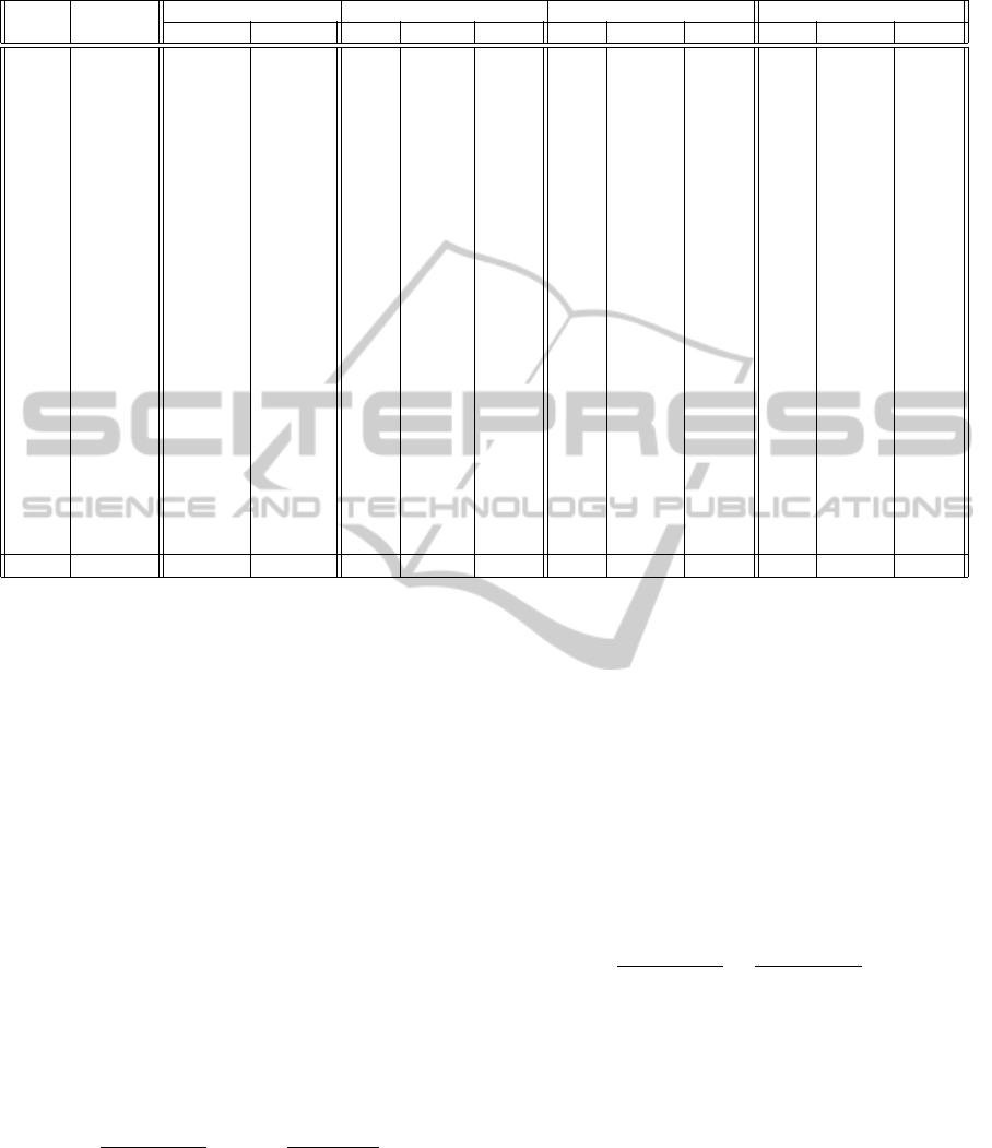
Table 1: Results of exact search, relaxations and randomized rounding.
Data Nb of Opt RelaxQP RelaxSDP RelaxSDP-Q
set bin. var. Obj Time Gap Time RR Gap Time RR Gap Time RR
D-1 215 3 343 1 0.73 0.02 2.35 0.54 12 2.35 0.26 12 0.70
D-2 278 3 254 21 0.80 0.00 3.88 0.64 19 1.49 0.46 21 1.70
D-3 341 3 174 183 0.94 0.02 4.86 0.82 31 2.43 0.65 36 3.25
D-4 406 3 110 1 286 1.10 0.02 4.23 0.97 44 5.04 0.83 54 5.14
D-5 469 3 051 7 200 1.18 0.02 11.70 1.08 63 3.72 0.96 79 4.04
D-6 530 2 994 5 780 1.17 0.03 14.56 1.09 81 3.35 1.00 108 4.73
D-7 215 3 297 2 1.24 0.02 3.31 1.03 5 2.82 0.68 6 0.82
D-8 278 3 223 8 1.89 0.03 10.28 1.72 8 7.15 1.38 11 3.35
D-9 341 3 176 39 2.94 0.08 11.31 2.81 15 9.95 2.49 64 2.11
D-10 406 3 133 169 3.91 0.13 14.69 3.80 26 11.94 3.52 98 8.98
D-11 469 3 070 76 3.87 0.18 13.56 3.78 38 13.81 3.53 147 11.79
D-12 530 3 024 232 4.25 0.20 14.47 4.17 53 17.98 3.95 236 16.20
D-13 539 12 580 7 200 0.85 0.05 3.16 0.77 154 3.28 0.61 171 2.08
D-14 698 12 431 7 200 0.95 0.10 3.47 0.89 252 3.76 0.76 286 4.06
D-15 852 12 290 7 200 1.13 0.14 5.78 1.08 373 4.58 0.99 436 4.83
D-16 1 011 12 156 7 200 1.14 0.14 6.16 1.09 578 5.19 1.02 750 5.29
D-17 1 170 12 034 7 200 1.15 0.22 5.72 1.12 791 5.77 1.08 1008 6.36
D-18 1 322 11 939 7 200 1.35 0.27 6.47 1.32 1030 5.67 1.30 1308 7.00
D-19 537 12 679 7 200 1.21 0.16 2.80 1.16 68 2.95 1.07 310 4.48
D-20 695 12 464 7 200 1.57 0.54 5.96 1.52 137 6.56 1.44 447 6.31
D-21 853 12 289 7 200 1.98 0.94 9.28 1.94 242 8.91 1.85 805 6.74
D-22 1 008 12 159 7 200 2.37 1.90 9.15 2.33 382 7.47 2.27 1113 8.80
D-23 1 165 12 034 7 200 2.65 2.95 7.87 2.62 628 7.70 2.58 2106 6.86
D-24 1 316 11 915 7 200 2.87 3.65 10.93 2.84 823 9.89 2.80 2231 8.52
Av. 651.83 7700.85 4224.91 1.80 0.49 7.75 1.71 243.88 6.41 1.56 493.46 5.59
• Opt: the best solution found within the time limit
(2 hours) by using CPLEX-Quadratic 12.1. The
time value7200 means that the time limit has been
reached, so the obtained integer solution is not op-
timal ;
• RelaxQP: the continuous relaxation computed
with CPLEX-Quadratic 12.1;
• RelaxSDP: the SDP relaxation computed with the
SDP solver CSDP 6.1.1 (cf (Borchers, 1999));
• RelaxSDP-Q: the SDP relaxation computed with
CSDP 6.1.1 with quadratic cuts (cf 3.3) ;
For each data set, the table 1 reports the number of
binary variables, the value of the objective function
(in currency unit), the computational time in second
and, for each kind of relaxation, the associated gap
(Gap) and the relative gap of the randomized rouding
(RR), whose formula are given below. The last line
(Av.) gives the average of the previous lines.
Gap =
p
opt
− p
relax
p
relax
RR =
p
RR
− p
opt
p
opt
(17)
Analysis of the Results
First we observe that CPLEX reaches the limited time
for relatively small instances (e.g. 469 binary vari-
ables). This is in line with our expectations that this
kind of problem is very hard for CPLEX, despite a
quite small gap attained with continuous relaxation.
This may be related to the fact that, due to the
demand constraint, the variable part of the objective
function is very small w.r.t the absolute value of the
cost. In other words, the optimal value is high, even
with a ”perfect” outages scheduling. Let’s denote P
the best possible objective value for a given data set,
computed by considering the largest possible search
space, and let’s consider the variable part of the ob-
jective function, that is p − P, if p is the objective
value. Then, the gap would increase, as shown in the
following formula:
p
opt
− p
relax
p
relax
− P
>
p
opt
− p
relax
p
relax
(18)
This illustrates the importance of considering the
relative improvement of the gap achieved by semidef-
inite relaxation, rather that its absolute value.
For example, on the data set D-1, the gap is almost
divided by three. Unfortunately, this ratio decreases
as the number of binary variables raises, whereas the
gap increases. This can be explained by the fact that
the ”exact solution” provided here is not optimal, con-
sidered that the computational time of CPLEX is lim-
ited. Let’s denote p
′
opt
> p
opt
this value: then the ra-
tio computed with this value is greater than the ratio
computed with p:
ICORES 2012 - 1st International Conference on Operations Research and Enterprise Systems
390

p
opt
− p
relaxCPLEX
p
opt
− p
relaxSDP
>
p
′
opt
− p
relaxCPLEX
p
′
opt
− p
relaxSDP
(19)
On average, the gap improves from 1.80% to
1.71% with original SDP relaxation and 1.56% with
addition of valid equalitites. This latter improve-
ment is promising, even though it comes at high ad-
ditional computational cost, particularly on the larger
instances. This can be ascribed to the fact that SDP
solvers are only in their infancy, especially compared
to a commercial solver like CPLEX.
Finally, the randomized rounding yields satisfying
results: due to the random aspect of the procedure,
there are still some data set where the continuous re-
laxation gives better results than the semidefinite re-
laxation, but on average the loss of optimality reduces
from 7.75% to 6.41% and 5.59%, which is significant
when considering the huge amount at stake.
5 CONCLUSIONS AND
PROSPECTS
We investigated in this paper, semidefinite relaxations
for a MIQP (Mixed-Integer Quadratic Program) ver-
sion of the scheduling of nuclear power plants out-
ages. Comparison of the results obtained on signifi-
cant data sets shows the following main results. First,
our MIQP is extremely hard to solve with CPLEX.
Second, semidefinite relaxations provide a tighter
convex relaxation than the continuous relaxation. In
our experiments the gap between the optimal solu-
tion and the continuous relaxation is on average equal
to 1.80% whereas the semidefinite relaxation yields
an average gap of 1.56%. Third, the computational
time for computing these semidefinite relaxations is
reasonable. Exploiting those results in a randomized
rounding procedure instead of the result of the contin-
uous relaxation leads to a significant improvement of
the feasible solution.
In the view of these preliminary results, additional
investigations will concern i) introduction of more
valid inequalities, ii) evaluation of others SDP resolu-
tion techniques, for instance Conic Bundle for facing
problems of huge size.
REFERENCES
Borchers, B. (1999). Csdp, a C library for semidefinite pro-
gramming.
Helmberg, C. and Rendl, F. (2000). A spectral bundle
method for semidefinite programming. SIAM Journal
on Optimization, 10(3):673–696.
Helmberg, C., Rendl, F., Vanderbei, R. J., and Wolkowicz,
H. (1996). An interior-point method for semidefinite
programming. SIAM Journal on Optimization, 6:342–
361.
Khemmoudj, M. O. I., Bennaceur, H., and Porcheron,
M. (2006). When constraint programming and local
search solve the scheduling problem of electricit´e de
france nuclear power plant outages. In 12th Interna-
tional Conference on Principles and Practice of Con-
straint Programming (CP’06), pages 271–283. LNCS.
Laurent, M., , , and Rendl, F. (2005). Semidefinite program-
ming and integer programming. In K. Aardal, G. N.
and Weismantel, R., editors, Handbook on Discrete
Optimization, pages 393–514.
Porcheron, M., Gorge, A., Juan, O., Simovic, T., and
Dereu, G. (2009). Challenge roadef/euro 2010: A
large-scale energy management problem with var-
ied constraints. Technical report, EDF R&D.
http://challenge.roadef.org.
Sherali, H. D. and Adams, W. P. (1990). A hierarchy of
relaxations between the continuous and convex hull
representations for zero-one programming problems.
SIAM Journal on Discrete Mathematics, 3(3):411–
430.
Todd, M. J. (2001). Semidefinite optimization. Acta Nu-
merica, 10:515–560.
Vandenberghe, L. and Boyd, S. (1994). Semidefinite pro-
gramming. SIAM Review, 38:49–95.
Wolkowicz, H., Saigal, R., and Vandenberghe, L., editors.
Handbook of Semidefinite Programming: Theory, Al-
gorithms, and Applications, volume 27.
SEMIDEFINITE RELAXATIONS FOR THE SCHEDULING NUCLEAR OUTAGES PROBLEM
391
