A COMBINED UNIFORM AND HEURISTIC SEARCH ALGORITHM

FOR MAINTAINING SHORTEST PATHS ON FULLY DYNAMIC

GRAPHS

Sandro Castronovo

, Bj

orn Kunz

and Christian M

uller

1,2

German Research Center for Artiﬁcial Intelligence (DFKI), Campus D3.2, Saarbr

ucken, Germany

Action Line Intelligent Transportation Systems, EIT ICT labs, Saarbr

ucken, Germany

Keywords:

Graph theory, Dynamic graphs, Heuristic search, Shortest paths.

Abstract:

Shortest-path problems on graphs have been studied in depth in Artiﬁcial Intelligence and Computer Science.

Search on dynamic graphs, i.e. graphs that can change their layout while searching, receives plenty of attention

today – mostly in the planning domain. Approaches often assume global knowledge on the dynamic graph, i.e.

that topology and dynamic operations are known to the algorithm. There exist use-cases however, where this

assumption cannot be made. In vehicular ad-hoc networks, for example, a vehicle is only able to recognize

the topology of the graph within wireless network transmission range. In this paper, we propose a combined

uniform and heuristic search algorithm, which maintains shortest paths in highly dynamic graphs under the

premise that graph operations are not globally known.

1 INTRODUCTION

Shortest path problems on graphs have been thor-

oughly studied in Artiﬁcial Intelligence and Com-

puter Science literature. Single-source shortest path

or all-pair shortest path problems with positive edge

weights can be solved using widely known algo-

rithms, such as Dijkstra (Dijkstra, 1959) and A*.

There are a large number of applications: modern

navigation systems, for example, use implementa-

tions of these algorithms for route planning, network

protocols use them in order to route data packets from

one physical location to another and many planning

systems in Artiﬁcial Intelligence use variants of these

algorithms.

The problem becomes signiﬁcantly more chal-

lenging when we allow certain dynamic operations on

the graph while searching, such as insertions or dele-

tions of vertices as well as changes of edge weights.

This problem drew attention of research in Artiﬁcial

Intelligence and related Computer Science ﬁelds. Ap-

proaches by (Nannicini and Liberti, 2008; Koenig

et al., 2004; Misra and Oommen, 2004; Cicerone

et al., 2003; Demetrescu and Italiano, 2003; Frigioni

et al., 2000) among others assume global knowledge

on the performed graph operations. This means they

are only applicable on graphs, for which the topol-

ogy and all executed operations are known at every

point in time. (Koenig et al., 2004), for example, as-

sume that every vertex stores its distance to a start

vertex of a shortest path. They modify this informa-

tion on every graph operation and use the result for

re-calculating. Work by (Misra and Oommen, 2004)

transfers the problem into the domain of Learning Au-

tomata but also allows access to the entire topology of

the dynamic graph.

There exist applications, however, in which this

knowledge can neither be assumed nor derived. Con-

sider a vehicular ad-hoc network, for example, where

vertices are vehicles, edges are wireless connections

between two vehicles, the task is to send data from

car A to car B, and B is not in A’s transmission range.

While searching a path to B, all of the operations

above can occur in arbitrary order and number, be-

cause the topology of the underlying graph is subject

to fast deletion and insertions of vertices and the algo-

rithm has no information about these changes. Hence,

we look at a ”fully dynamic problem” (Dynamic Sin-

gle Source Shortest Path Problem, or DSSSP). In our

example, the dynamic operations may even break the

connection between vertices. Furthermore, it is not

efﬁcient and sometimes even not feasible to visit ev-

ery vertex after a graph operation. Network band-

width is considered a limited resource in vehicular

ad-hoc networks, which is also a reason why the cited

algorithms are not applicable here.

119

Castronovo S., Kunz B. and Müller C..

A COMBINED UNIFORM AND HEURISTIC SEARCH ALGORITHM FOR MAINTAINING SHORTEST PATHS ON FULLY DYNAMIC GRAPHS.

DOI: 10.5220/0003743401190126

In Proceedings of the 4th International Conference on Agents and Artiﬁcial Intelligence (ICAART-2012), pages 119-126

ISBN: 978-989-8425-95-9

 2012 SCITEPRESS (Science and Technology Publications, Lda.)

In this paper, we propose a combined uniform and

heuristic search algorithm, which is able to solve the

single-source shortest path problem under unknown

topology changes in fully dynamic graphs. In order

to do so we instantiate two graphs: The ﬁrst, G =

(V, E), is static. We solve the single-source shortest

path problem on G using Dijkstra’s algorithm. The

second,

G = (

V ,

E), is subject to the described graph

operations. We then exploit domain speciﬁc relations

between the two graphs and approximate the shortest

path identiﬁed on G in

G. Our algorithm only depends

on local information about graph operations in order

to heuristically maintain or alter the initial path found

in G.

2 RELATED WORK

(Koenig et al., 2004) propose an incremental ver-

sion of the popular A* algorithm based on a dynamic

gridworld. This world consists of cells which de-

note vertices. Edges are drawn between neighbour-

ing cells. The algorithm continously ﬁnds shortest

paths between a start cell s

start

and a goal cell s

goal

Their approach is incremental since they reuse results

from previous searches. However, they assume global

knowledge about the gridworld: The algorithm holds

data structures for the start distance of every cell as

well as a list of traversable and blocked cells. In our

application domain this assumption cannot be made.

The approach of (Misra and Oommen, 2004)

transfers the DSSSP problem into the domain of

Learning Automata. They establish three compo-

nents: The learning automaton (LA), which is in-

stantiated in every vertex, the random environment

(RE) and a penalty/reward system. RE changes edge

weights using stochastic information and LA con-

stantly interacts with this environment by guessing

whether or not a node belongs to the shortest path.

The LA constantly receives rewards or penalties de-

pending on whether its guess was right or not. Al-

though the distribution of the weight changes by the

RE are unknown to LA, it is allowed to retrieve a

snapshot of the whole graph and its current edge

weights. Basically, this snapshot, Dijkstra’s algorithm

and the received penalities/rewards are used for short-

est path computation. It is obvious that in our domain

such a snapshot of the whole graph is not available.

(Frigioni et al., 2000) propose fully dynamic al-

gorithms for solving DSSSP by counting the vertices

affected by changes of the graph. When increasing

the weight of an edge, the affected vertices are those

which change the distance from the start vertex. The

algorithm marks vertices according to their status af-

ter a graph operation; White marked vertices were

not affected by an operation. Neither the distance

from the source nor the parent in the shortest path

tree changed. Red marked vertices increased their

distance from the source while the distance of the

ones marked pink remained constant but it replaces

the old parent in the shortest path tree. Obviously,

this approach also relies on global knowledge about

the graph topology and the operations on it.

(Seet et al., 2004) (SEET) and (Granelli et al.,

2007) (GRANELLI) are both routing protocols for ve-

hicular ad-hoc networks. Both implementations have

to solve the single-source shortest path problem in dy-

namic graphs having no knowledge about its topol-

ogy by the very nature of their application domain.

The approach by (Seet et al., 2004) is to employ two

graphs: One ﬁxed, one dynamic. There exists a con-

nection between the two in a way such that the topol-

ogy of the ﬁxed graph correlates with the dynamic

one. By solving the SSSP on the ﬁxed graph they

try to approximate this path in the dynamic one. We

adopt this idea but also take local information about

graph operations into account allowing us to dynami-

cally assign lower weights to edges in the ﬁxed graph

for solving the SSSP. This allows our algorithm to

adapt the path on the static graph according to the lo-

cally known changes in the dynamic one.

The key idea behind (Granelli et al., 2007) is to

estimate the topology of the dynamic graph by using

information about the neighbouring vertices. More

precisely they try to estimate the position of neigh-

bouring vehicles by using their respective velocity

and direction vector. Our approach also assumes cer-

tain knowledge, e.g. the route on the map a vehicle

is driving along, about the surrounding topology of a

given vertex (see Section 3) thus allowing us more ac-

curate position information since we can also take the

curvature of a street into account by computing the

position along it.

3 SHORTEST PATH

COMPUTATION UNDER

UNKNOWN GLOBAL GRAPH

OPERATIONS

Let G = (V, E) be a weighted, directed graph, which

is ﬁxed, i.e., no insertions and deletions are allowed.

The topology of G is known to the algorithm. Fur-

thermore,

G = (

V ,

E) denotes a fully dynamic graph.

N is a list containing all vertices, which are reachable

from a vertex ˜v ∈

G with distance 1 (direct connec-

tion by one edge). Only the vertices in

N are known

ICAART 2012 - International Conference on Agents and Artificial Intelligence

120

to the algorithm. The remaining topology of

G is hid-

den: Neither the number of vertices is known nor the

edges between them. In order to give the reader a

clear understanding of these notions, Figure 1 exem-

pliﬁes these terms when applied to the domain of ve-

hicular ad-hoc networks: Our algorithm is running on

green Vehicle 1. Black points mark vertices v ∈ G,

here: junctions. Connecting lines in between mark

edges e ∈ G (streets). All vehicles in light blue are lo-

cated within transmission range and thus are elements

of list

N. Vehicles form vertices of dynamic graph

G. Dotted lines between them mark edges ˜e ∈

G, e.g.

wireless connections. Note, that there is no (direct)

edge between vehicle 1 and black vehicles 6,7 and 8

since they are out of transmission range.

Figure 1: Notations used throughout the paper on the exam-

ple of vehicular ad-hoc networks.

We deﬁne a set of functions that can be queried by

every vertex in

1. A function

f :

V × T → E × R

maps a vertex

˜v ∈

G to exactly one edge e ∈ E. Moreover, it

generates a virtual edge between the vertex ˜v and

the start vertex of the assigned edge e and sets a

weight depending on the speciﬁc application do-

main. For example, we can interpret this as the

distance vehicle ˜v travelled along a road e.

f up-

dates this mapping and weight in speciﬁc time in-

tervals thus enabling the algorithm to see a snap-

shot of the neighbouring topology of

G at a point

in time t ∈ T . Hence, a request to

f requires a

time t ∈ T. Note, that a vertex ˜v ∈

G is only al-

lowed to query vertices in

N, which contains di-

rect neighbours within transmission range. Fur-

thermore, queries to future edge weights return

null. Also note, that the dynamic graph changes

very quickly and

f only provides a snapshot of

the neighbouring topology of

2. A function w : V ×

V × T → R

returns a weight

of a virtually drawn edge between a vertex in

and a vertex in G. Only queries to elements in

are allowed since the knowledge in a vertex ˜v ∈

is restricted to its direct neighbours. In contrast

to the virtual edge in

f for vehicular ad-hoc net-

works this gives us the euclidian distance of a ve-

hicle ˜v ∈

V to a crossing v ∈ V .

3. A function ˜g :

V → List < E > maps every ˜v ∈

to a sequence of edges e

, ..., e

∈ E effectively

describing the path of ˜v on G. In vehicular ad-hoc

networks this maps to the most probable path of a

vehicle.

After solving the SSSP on ﬁxed graph G yielding

shortest path P, the algorithm’s task is now to approx-

imate P in

G by making use of the information avail-

able from the deﬁned functions

f ,w and ˜g. In the fol-

lowing, we denote the aproximated shortest path as

Note, that P is an array of vertices in G (in ascending

order).

Our algorithm is divided into seven steps, which

are summarized in Table 1. First, we check if the des-

tination vertex

d ∈

V is a direct neighbour, e.g. an

element in

N. In this case, no shortest path compu-

tation is necessary and the algorithm terminates after

adding ˜v to

If the destination vertex is not contained in

N, we

proceed with solving SSSP on G using a modiﬁed Di-

jkstra: Our Dijkstra implementation takes the number

of mappings of all ˜v ∈

N by ˜g to edges in G into ac-

count (as far this can be determined by the vertices

contained in

N and queries to ˜g). It assigns lower

weights on edges in G where density of mappings

is higher. This is done before every vertex decision

for

P to accomodate fast topology changes within the

graph.

We then estimate future edge weights of all ver-

tices in

N to the start vertices of their mapped edge

in G. This is especially necessary at low update rates

f to the vertices in

N. Since our application do-

main are vehicular ad-hoc networks we have to con-

sider this fact. A car traveling by 36 m/s on a motor-

way covers a substantial amount of a car’s transmis-

sion range between two position updates. Hence an

update by

f could delete an edge in

The following three steps are crucial for the algo-

rithm since the decision on next vertex for

P depends

on them. Every vertex in

N gets assigned three heuris-

tics within the interval of [0, 1] where higher values

denote higher priority in selecting the next vertex for

P. The three heuristics are given in Table 1, rows 4 –

A COMBINED UNIFORM AND HEURISTIC SEARCH ALGORITHM FOR MAINTAINING SHORTEST PATHS ON

FULLY DYNAMIC GRAPHS

121

Table 1: High level steps and actions of the search algo-

rithm.

# Step Action(s)

1 Check necessitiy

of Single Source

Shortest Path

computation

Check if a ˜v ∈

N is a destina-

tion. Add ˜v to

P and termi-

nate if true or continue other-

wise

2 Solve single-source

shortest path prob-

lem on G

Change weights of edges in

G according to number of

mappings of vertices ∈

to edges ∈ G. Use Dijk-

stra’s Algorithm to compute

the shortest path from source

to destination

3 Update neighbour

weights

Calculate estimated weights

∀ ˜v ∈

N to the start vertex of

their mapped edges in G

4 Calculate edge

weights between

v ∈ P and ˜v ∈

Prefer vertices with minimal

edge weight between virtu-

ally drawn edges between

vertices v ∈ P and vertices

˜v ∈

N. Weight the result with

predeﬁned α

5 Calculate mappings

of ˜v ∈

N with with

edges in P

Prefer vertices whose map-

ping by

f is close to edges in

P over others. Weight the re-

sult with predeﬁned β

6 Calculate edge

weights along P

Prefer vertices in with larger

sum of edge weights on P be-

fore others. Weight the result

with predeﬁned γ

7 Update

P Select a vertex ˜v ∈

N accord-

ing to computed heuristics in

steps 4 – 6 and add it to

P or

wait until next update from f

N if no vertex can be se-

lected. Repeat steps 1 – 7 un-

til destination reached

Each heuristic is multiplied by a weight of α, β

and γ respectively. The computations of the three

heuristics are described in detail below. The ﬁnal step

is to select a vertex in

N for

P based on the heuris-

tics computed in the steps before or restart the algo-

rithm on the vertex until we have have reached a ver-

tex close to destination vertex d.

Estimating Future Weights. The procedure for es-

timating future weights is given in Algorithm 1. Since

f updates

N only in speciﬁc intervals and the topol-

ogy of

G changes very quickly we try to estimate the

topology of the neighbouring vertices in

G. The idea

is to query

f on the edge weights of all vertices con-

tained in

N at time t and t − 1. We then use the delta

of the two weights and add it to the current weight of

a vertex in

N. We have to distinguish two cases here:

(1) At time t and time t

t−1

vertex ˜v maps to the same

edge in G, (2) At time t and time t

t−1

vertex ˜v maps to

different edge in G (line 4). This inﬂuences how ∆w

is calculated (lines 5 – 10).

If the estimated edge weight is larger than the

weight of the currently assigend edge of ˜v we do not

only estimate the weight, we also set the future as-

signed edge of ˜v using ˜g.

We store the updated values directly in ˜v.

Algorithm 1: Estimate future edge weights.

1: for all (˜v ∈

N) do

2: w

←

f ( ˜v,t).w

3: w

t−1

←

f ( ˜v,t

t−1

).w

4: if (

f ( ˜v,t).e ==

f ( ˜v,t

t−1

).e) then

5: ∆w ← w

− w

t−1

6: w

est

← w

+ ∆w

7: else

8: w

t−1

←

f ( ˜v,t

t−1

).e.w −

f ( ˜v,t

t−1

).w

9: ∆w ← w

+ w

t−1

10: w

est

← w

+ ∆w

11: end if

12: if (w

est

f ( ˜v,t).e.w) then

13: E ← ˜g( ˜v)

14: for (i ← 0; i < E.length − 1; i + +) do

15: if (E[i] ==

f ( ˜v,t).e) then

16: ˜v.e ← E[i + 1]

17: ˜v.w ← w

est

− E[i].w

18: end if

19: end for

20: else

21: ˜v.w ← w

est

22: end if

23: end for

Heuristic 1: Edge Weights between v ∈ P and ˜v ∈

N. Alogrithm 2 shows how the ﬁrst heuristic is com-

puted for selecting the next vertex for

P. The idea here

is to use w in order to identify the vertex ˜v ∈

N with

minimum weight to a vertex v ∈ P. It is obvious to

prefer these edges for

P since they come close to the

initial found path P.

The code is executed for ∀ ˜v ∈

N from the previ-

ous step and computes ∀v ∈ P the weight of an edge

between a vertex ˜v ∈

G to a vertex v ∈ G (line 4-

7). We only consider vertices up to a certain weight

max

. (lines 8-10). Heuristic 1 is then deﬁned as

= α ∗ (1 −

max

) (line 11). Remember, that higher

values denote higher priority in selecting the next ver-

tex for

P. Heuristic 1 is optimizing the stability of the

path

P since it prefers vertices ˜v ∈

V that are close to

the path vertices in P. In vehicular ad-hoc networks

we can interpret this as prefering vehicles that are on

street junctions which form natural turning points in

the street graph.

ICAART 2012 - International Conference on Agents and Artificial Intelligence

122

Algorithm 2: Heuristic 1: Edge weights between v ∈ P and

˜v ∈

1: for all ( ˜v ∈

N) do

2: w ← ∞

3: for all (v ∈ P) do

4: if (w(v, ˜v, t) < w) then

5: w ← w(v, ˜v, t)

6: end if

7: if (w > w

max

) then

8: w ← w

max

9: end if

10: end for

11: ˜v.h

← α ∗ (1 −

max

)

12: end for

Heuristic 2: Mappings of ˜v ∈

N with Edges in P.

Heuristic 2 is computed as stated in algorithm 3. As

for heuristic 1, the code is executed ∀ ˜v ∈

N. It scores

vertices in

N higher whose mappings to edges in G

matches more edges in P over others. Furthermore,

we take the direction of the edge into account: An

exact match gets assigned a score of ω. If the mapped

edge of ˜v is the opposite of an edge in P we assign

τ. If no match is detected, we assign a score of 0.

Note, that we require ω > τ. The actual values used

for evaluation are given in table 2.

Score

max

is deﬁned as

∑

|P|−1

i=0

ω. Heuristic 2 is de-

ﬁned as β ∗

score

max

, yielding to a value in the range

[0, 1] where larger values denote higher priority in se-

lecting the next vertex for

P. Finally, we assign the

weight β and store heuristic h

in ˜v (line 14). Heuris-

tic 2 is trying to optimize path stability by prefering

˜v ∈

V whose own path along G covers more of path

P, the idea being that if ˜v cannot ﬁnd next vertex for

P it at least gets closer to the destination. In vehicular

ad-hoc network terms we can interpret this as prefer-

ing a vehicle that can carry the message closer to the

destination in the case when a more suitable vehicle

cannot be found.

Heuristic 3: Edge Weights along P. The pseu-

docode for the third heuristic is given in Algorithm

4. It favours vertices in

N with larger sum of edge

weights on P before others. We ﬁrst look at the cur-

rent mapping of vertex ˜v ∈

N to an edge in G and

distinguish two cases:

• P contains the Current Mapping. We add up

the weight of edges e ∈ P starting from P[0] to the

current mapping of ˜v (lines 5-13)

• P doesn’t Contain the Current Mapping. We

add up the weight of every edge e ∈ P until the

vertex with the least weight from ˜v to a vertex v ∈

P (lines 15-30)

Algorithm 3: Heuristic 2: Mappings of ˜v ∈

N with with

edges in P.

1: for all ( ˜v ∈

N) do

2: currentScore ← 0

3: for (i ← 0; i < P.size − 2; i + +) do

4: p

← P[i]

5: p

← P[i + 1]

6: if (edge(p

, p

) ∈ ˜g( ˜v)) then

7: currentScore ← currentScore + ω

8: else

9: if (edge(p

, p

) ∈ ˜g( ˜v)) then

10: currentScore ← currentScore + τ

11: end if

12: end if

13: end for

14: ˜v.h

← β ∗ (

currentScore

score

max

)

15: end for

Like before, we calculate a heuristic in the interval

(0,1) We multiply by a weight of γ (line 31). Also

here, larger values denote higher priority in selecting

the next vertex for

P. In constrast to heuristic 1 and

2 this heuristics tries to optimize progress towards the

destination by choosing the next vertex ˜v ∈

V that is

furthest along P. In vehicular ad-hoc networks this

means choosing the vehicle furthest along the guiding

path on the street map.

Selecting the Next Vertex for

P. After calculating

the heuristics described in the previous sections we

can now select a vertex in

N for

P. Let H be the

set containing the sums of h

, h

∀n ∈

N. Then,

the next vertex for

P is deﬁned as the vertex with the

largest sum in H.

If the next vertex is

P.length − 1] we re-calculate

after the next update of

f .

4 EVALUATION

We integrated our algorithm into the transportation

layer of a network stack and performed a simple

point-to-point sending task in a simulator for evalu-

ation of vehicular ad-hoc network applications (V2X

Simulation Runtime Infrastructure or short VSimRTI

(N. Naumann, 2009)). VSimRTI integrates and co-

ordinates different simulators and constitutes a mid-

dleware between the individual simulators. For re-

alistic simulation we used the wireless network sim-

ulator Jist/Swans (Barr et al., 2005) and the trafﬁc

simulation SUMO (Krajzewicz et al., 2002). We fur-

thermore integrated the effect of buildings on wireless

transmission into the simulator. Two vehicles are only

A COMBINED UNIFORM AND HEURISTIC SEARCH ALGORITHM FOR MAINTAINING SHORTEST PATHS ON

FULLY DYNAMIC GRAPHS

123

Algorithm 4: Heuristic 3: Edge weights along P.

1: w

← P.totalWeight

2: for all ( ˜v ∈

N) do

3: e

˜v

←

f ( ˜v,t).e

4: w ← 0

5: if (e

˜v

∈ P) then

6: for (i ← 0; i < P.size − 2; i + +) do

7: if (e

˜v

== edge(P[i], P[i + 1])) then

8: w ← w +

f ( ˜v,t).w

9: break

10: else

11: w ← w + edge(P[i],P[i + 1]).w

12: end if

13: end for

14: else

15: leastWeight ← ∞

16: v ← nil

17: for (i ← 0; i < P.size − 1; i + +) do

18: if (w(P[i], ˜v, t) < leastWeight) then

19: leastWeight ← w(P[i], ˜v, t)

20: v ← P[i]

21: end if

22: end for

23: for (i ← 0; i < P.size − 2; i + +) do

24: if (P[i] == v) then

25: break

26: else

27: w ← w + edge(P[i],P[i + 1]).w

28: end if

29: end for

30: end if

31: ˜v.h

← γ ∗ (

)

32: end for

able to communicate if and only if there is a line of

sight between them. This serves as a lower bound on

the connection between the vehicles in the network

simulator.

We compare the performance of our algorithm

with SEET (Seet et al., 2004) and GRANELLI

(Granelli et al., 2007) in terms of path discovery ra-

tio (PDR) and path discovery time (PDT). The ﬁrst

metric measures the ratio

PDR =

Success f ulShortestPathDiscoveries

TotalShortestPathSearches

and the second indicates time from beginning to end

of shortest path search PDT = t

end

−t

start

4.1 Implementation of

f , w and ˜g

Remember that graph G = (V, E) is represented by

the underlying city map. Junctions are vertices v ∈ V ,

road segments denote edges e ∈ E.

G = (

V ,

E) is

spanned by the vehicular ad-hoc network. Vehicles

are represented by ˜v ∈

V , edges ˜e ∈

E are considered

as wireless connection between two vehicles. The ab-

stract deﬁned functions

f , w and ˜g of Section 3 are

then implemented as follows: Given a time t,

f as-

signs vehicles to speciﬁc road segments. Weight is

calculated out of the distance to the beginning of the

assigned road segment. In our application domain,

f is responsible for controlling and updating posi-

tions of vehicles therefore realizing vehicle move-

ments over time. Function w returns the distance be-

tween a vehicle in transmission range and a junction

of the city map. The vehicles further include the road

segments which they have passed as well as their most

probable path in their position updates. This realizes

function ˜g.

4.2 Scenario

Evaluation was done in a scenario where every vehi-

cle starts one shortest path computation to a given car,

e.g. the center of the underlying city map. The des-

tination car remained stationary while all others were

driving a route on the map.

We optimzed weights for heuristics 1 – 3 introduced

in Section 3 on a randomly generated map shown in

Figure 2 (left). Weights and values for ω and τ, which

were found to be optimal for our algorithm, are given

in Table 2. We optimized for high PDR.

Figure 2: Fixed graphs used for parameter optimization and

evaluation. Left: Random generated, used for parameter

optimization (1200m x 1200m). Right: Graph generated

based on an existing road network of the city of Heidelberg,

Germany used for evaluation (1200m x 1200m).

After optimization, evaluation was done on a map

generated out of an existing city environment (Heidel-

berg, Germany, Figure 2, right). Evaluation runtime

was 120 seconds where we started shortest path com-

putation after 20 seconds simulation time. This en-

sured a fair distribution of vehicles on the map. n ve-

hicles per second were placed on the map by the sim-

ulator and removed after they completed their route

where n ∈ {1, 2, 3, 4}. For n = 1 this resulted in 120

path computations. We repeated every run three times

for every n and algorithm. This means 120 ∗ 3 = 360

path computations for n = 1 in total per algorithm and

720, 1080, 1440 for n = 2, 3, 4 respectively resulting

in a total of 3600 path searches per algorithm.

ICAART 2012 - International Conference on Agents and Artificial Intelligence

124

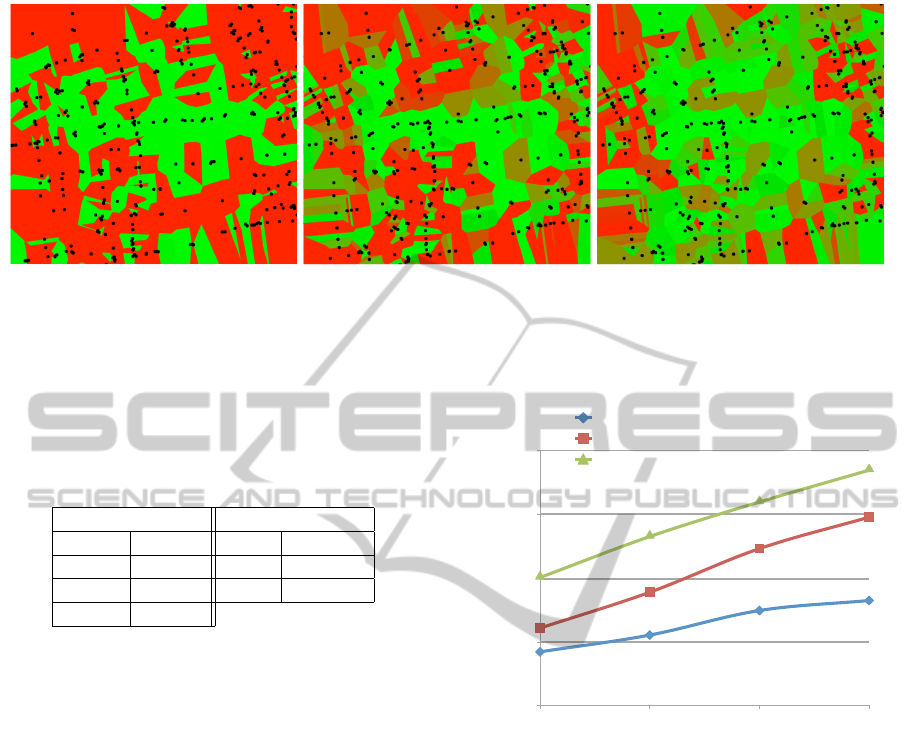
Figure 3: Voronoi diagrams visualizing PDR and PDT. Dots mark nodes in which path computation started, color denotes

average time until shortest path completed in the enclosed region. Left: GRANELLI (n = 4), fast but unreliable; middle: SEET

(n = 4), slower but more reliable than GRANELLI due to taking correlation of

G and G into account; right: Our approach,

n = 4, taking correlation between

G and G as well as local information on dynamic graph operations into account outperforms

GRANELLI and SEET.

Table 2: Values of the various weights used during the eval-

uation. The three on the left side denote the weights for the

different heuristics while the two on the right were used for

score computation of Heuristic 2 (see Algorithm 3).

Heuristic Weight Heuristic 2 score

weight value score value

α 0.5 ω 2

β 0.3 τ 1

γ 0.2

4.3 Results and Analysis

Results in Figure 4 and Figure 5 show that our ap-

proach outperforms SEET and GRANELLI in means

of PDR. As expected, PDR increases with increas-

ing trafﬁc density. SEET obviously beneﬁts from the

available information about the underlying city map

(the static graph G). GRANELLI lacks this kind of

information which results in a lower PDR. As our

approach also takes local information about graph

operations in

G (the vehicular ad-hoc network) into

account, it scores higher PDR than both SEET and

GRANELLI. The results are statistically signiﬁcant

(p < .001 according to a χ

test).

However, by means of PDT, GRANELLI is su-

perior to SEET and our approach. Both, SEET and

our approach re-schedule path searching in a vertex

when no suitable successor vertex could be identiﬁed

for the shortest path (see Section 3). GRANELLI’s

behaviour in such a situation is to greedily select

a next vertex out of the neighbouring vertices and

do no re-scheduling at all. This also justiﬁes low

PDR for GRANELLI. Interestingly, PDT increases for

GRANELLI but decreases for both SEET and our ap-

proach when there are more vehicles on the graph.

In this case both, SEET and our approach have an

0,23

0,45

0,68

0,90

120 240 360 480

GRANELLI

SEET

Our approach

Figure 4: Path Discovery Ratio (PDR) results for all three

algorithms. X-Axis gives the number of path searches, y-

axis gives the percentage of successful path searches. As

expected, PDR increases with a larger number of cars on

the evaluation scenario.

increased number of vertices available for choosing

the next vertex for the shortest path and the propa-

bility of ﬁnding a suitable one also increases since

re-computing time for heuristics is lower than the re-

scheduling interval PDT decreases in this case. Be-

cause our approach considers local information about

graph operations it superseeds SEET by means of

PDT over time which results in a lower number of

re-schedules.

Figure 3 depicts voronoi visualizations for all

three algorithms after a run with n = 4. Black dots

mark starting positions for shortest path computation.

Enclosing colored areas denote PDT to the centre of

the map for an individual path in ms (more red ar-

eas mark higher PDT). After a threshold of 15000 ms

path computation was stopped and marked as failed.

A COMBINED UNIFORM AND HEURISTIC SEARCH ALGORITHM FOR MAINTAINING SHORTEST PATHS ON

FULLY DYNAMIC GRAPHS

125

1500

3000

4500

6000

120 240 360 480

GRANELLI

SEET

Our approach

Figure 5: Path Discovery Time (PDT) for all three algo-

rithms. X-Axis gives the number of path searches, y-axis

gives the time in ms. GRANELLI does not reschedule when

no suitable successor vertex for the shortest path can be

found. By increasing the number of vertices in the graph,

PDT gets lower for SEET and our approach.

One clearly recognizes short PDT of GRANELLI but

low PDR: Paths are found quickly or not at all. Re-

scheduling in cases when no successor vertex for

the shortest path can be identiﬁed results in stepwise

PDTs. Results of our approach reﬂect high PDR even

for large path lenghts due to exploiting local informa-

tion on dynamic graph operations.

5 CONCLUSIONS

In this paper, we developed a combined uniform

and heuristic search algorithm for maintaining short-

est paths in fully dynamic graphs. While other

approaches assume global knowledge on performed

graph operations, we argued that there exist use cases

where this information is not available. Our approach

shows that in those cases the algorithms’ performance

can greatly beneﬁt from considering domain speciﬁc

knowledge. In our example, we instantiated two

graphs: A static and dynamic one. We exploited do-

main speciﬁc relations between these graphs in or-

der to heuristically maintain a shortest path in a dy-

namic graph. The used heuristics are also tailored

to the domain. We applied our approach to vehicu-

lar ad-hoc networks and integrated it into the trans-

portation layer of a network stack to use it for routing

data packets between two vehicles. Evaluation was

performed against two other routing algorithm of this

domain. Due to re-scheduling when no neighbouring

vertex could be identiﬁed during shortest path search,

the approach of GRANELLI is superior to our imple-

mentation in means of PDT. However, our approach

outperformed SEET and GRANELLI in means of PDR.

REFERENCES

Barr, R., Haas, Z. J., and van Renesse, R. (2005). Jist:

An efﬁcient approach to simulation using virtual ma-

chines. Software Practice & Experience, 35(6):539–

576.

Cicerone, S., Stefano, G. D., Frigioni, D., and Nanni, U.

(2003). A fully dynamic algorithm for distributed

shortest paths. Theoretical Computer Science, 297:1–

Demetrescu, C. and Italiano, G. F. (2003). A new approach

to dynamic all pairs shortest paths. In Proceedings

of the thirty-ﬁfth annual ACM symposium on Theory

of computing, STOC ’03, pages 159–166, New York,

NY, USA. ACM.

Dijkstra, E. W. (1959). A note on two problems in con-

nection with graphs. Numerische Mathematik, 1:269–

271.

Frigioni, D., Spaccamela, A. M., and Nanni, U. (2000).

Fully dynamic algorithms for maintaining shortest

path trees. Algorithms, 34(2):251–281.

Granelli, F., Boato, G., Kliazovich, D., and Vernazza, G.

(2007). Enhanced gpsr routing in multi-hop vehicular

communications through movement awareness. IEEE

COMMUNICATIONS LETTERS, 11(10):781–783.

Koenig, S., Likhachev, M., and Furcy, D. (2004). Lifelong

planning A*. Artif. Intell., 155:93–146.

Krajzewicz, D., Hertkorn, G., R

ossel, C., and Wagner, P.

(2002). Sumo (simulation of urban mobility); an

open-source trafﬁc simulation. In Proceedings of the

4th Middle East Symposium on Simulation and Mod-

elling.

Misra, S. and Oommen, B. J. (2004). Stochastic learn-

ing automata-based dynamic algorithms for the sin-

gle source shortest path problem. In Proceedings of

the 17th international conference on Innovations in

applied artiﬁcial intelligence, IEA/AIE’2004, pages

239–248. Springer Springer Verlag Inc.

N. Naumann, B. Schuenemann, I. R. (2009). Vsimrti - sim-

ulation runtime infrastructure for v2x communication

scenarios. In Proceedings of the 16th World Congress

and Exhibition on Intelligent Transport Systems and

Services.

Nannicini, G. and Liberti, L. (2008). Shortest paths on dy-

namic graphs.

Seet, B., Liu, G., Lee, B., Foh, C., and Wong, K.-J. (2004).

A-star: A mobile ad hoc routing strategy for metropo-

lis vehicular communications. In Lecture Notes in

Computer Science Vol. 3042: IFIP-TC6 Networking

Conference.

ICAART 2012 - International Conference on Agents and Artificial Intelligence

126