
NEW REASONING FOR TIMELINE BASED PLANNING
An Introduction to J-TRE and its Features
Riccardo De Benedictis and Amedeo Cesta
CNR, Italian National Research Council, ISTC, Rome, Italy
Keywords:
Planning, Scheduling, Reasoning on timelines.
Abstract:
Time and resource reasoning are crucial aspects for modern planners to succeed in several real world domains.
A quite natural way to deal with such reasoning is to use timeline based representations that have been ex-
ploited in several application-oriented planners. The search aspects of those planners still remain a “black
art” for few experts of such particular approach. This paper proposes a new model to conduct search with
timelines. It starts from the observation that current timeline based planners spend most search time in doing
blind constraint reasoning and explores a different hybrid model to represent and reason on timelines that may
overcome such computational burden.
1 INTRODUCTION
Temporal flexibility required in controlling mecha-
nisms in real-time (i.e., robotics), interacting with
agents requirements as well as uncertainty of real
world domains, are just some of the arguments that
are leading to the progressive exploration of different
planning methodologies (Erol et al., 1994; Ghallab
and Laruelle, 1994; Smith et al., 2000) and to the ex-
tensions of most classic ones (Fox and Long, 2003).
Timeline based planning constitutes an intuitive
alternative to classical planning approaches by iden-
tifying relevant domain components evolving in time.
Although attractive from a temporal flexibility point
of view, these kind of planners have to cope with per-
formance issues due to the complexity that derives
from their expressiveness. Most of their computa-
tional time (often up to 90% in complex domains) is
spent in temporal reasoning wasting time to maintain
a huge amount of information sometime only partially
useful (for example, the distance between time-points
of different timelines most of which are not used in
current problems). Furthermore, temporal networks
are always quite sparse so, complex methods inher-
ited from constraint-based scheduling literature (e.g.,
all-pair-shortest-path algorithms) may result too ex-
pensive in most cases. A further reason for slow-
down can be found in the management of states of
the search space. Common timeline based planners,
indeed, consider neighborhood states as completely
different problems although they are quite similar.
Imagine, for example, we have one hundred activ-
ities a
1
, a
2
, . . . , a
i
, . . . , a
j
, . . . , a
100
with some starting,
ending and duration constraint. Among these activi-
ties, we have two special activities a
i
and a
j
that we
know cannot overlap. Common planners, although
with some differences, would generate two nodes on
the search space having respectively a
i
≺ a
j
(hence-
forth we will use this formalism to indicate a prece-
dence constraint among elements) and a
j
≺ a
i
, each
representing a single constraint satisfaction problem
(CSP), and would solve them separately (we have,
basically, two all-pair-shortest-path problems). We
could merge these two states into a single state having
a a
i
≺ a
j
∨ a
j
≺ a
i
constraint. Although this example
addresses the weakness of common approaches, un-
fortunately it does not make clear why common plan-
ners do not make use of disjunctive CSPs. The reason
for this is that disjunctive CSPs still have to take care
of the causality in the domain so are, in general, not
enough for our planning needs.
Let us assume, for example, that every morning
we have to reach our work place starting from home.
In order to achieve the task we have two alternatives:
either take a bus or walk. In a timeline based planning
system we can model this simple problem by means
of a single state variable having four predicates as
possible values: AtHome(), TakeBus(), TakeWalk()
and AtWork(). A solution to a planning problem is
represented by a legal sequence of tokens (values as-
sumed over temporal intervals) defined on such state
variable. Let us assume that the initial state is de-
scribed by the token t
0
of value AtHome() satisfying
a relation start
at(t
0
, 0) (to say that the initial value
144
De Benedictis R. and Cesta A..
NEW REASONING FOR TIMELINE BASED PLANNING - An Introduction to J-TRE and its Features.
DOI: 10.5220/0003746901440153
In Proceedings of the 4th International Conference on Agents and Artificial Intelligence (ICAART-2012), pages 144-153
ISBN: 978-989-8425-95-9
Copyright
c
2012 SCITEPRESS (Science and Technology Publications, Lda.)

starts at time 0) and let us fix AtWork() as our cur-
rent goal. Additionally, we know that any AtWork()
proposition requires to be met by a TakeBus() propo-
sition or by a TakeWalk() proposition. Furthermore
both TakeBus() and TakeWalk() require to be met by
an AtHome() proposition but TakeBus() requires a
duration [15, + inf] while TakeWalk() requires a du-
ration [30, 40]. This is the basic way of specifying
causality with timelines.
In order to solve this simple problem, a timeline-
based planner would generate two nodes on the
search space having respectively a TakeBus() and a
TakeWalk() proposition, both generated to achieve
the AtWork() goal. Each node would represent a sin-
gle CSP to be solved separately in order to define start
and end times for all the values of the state variable.
Alternatively, we could create a single node having a
TakeBus() ∨ TakeWalk() clause. Solving constraints
of this node, now, would solve our entire planning
problem. Notice that enabling the TakeBus() (or the
TakeWalk()) value would also require to enable its
duration constraint and, if any, every consequence of
the presence of the TakeBus() (or TakeWalk()) fact
as, for example, a resource consumption due to ticket
payment.
In general, in this paper we explore the idea
of maintaining different states of the search space
through a single “extended CSP” that is expressive
enough to handle causal relations among its elements.
In so doing, we make the representation of search
space implicit hence simplifying the solver imple-
mentation phase and delegating all search aspects to
our extended CSP solver. We can reach these results
by modifying a common SAT solver (Een and Sorens-
son, 2003) and integrating it with a CSP solver. We
will then let the SAT solving procedure to guide all
the search process of both SAT and CSP problems in
a Satisfiability Modulo Theory (SMT) fashion – e.g.,
(Sebastiani, 2007).
This paper presents J-TRE (for Java Timeline Rea-
soning Environment) a new timeline based planning
and scheduling environment that puts our ideas into
practice. It is organized as follows: Section 2 con-
tains the basic terminology of timeline based reason-
ing, Section 3 presents the new proposal for modeling
the solution space and Section 4 describe an associ-
ated search procedure. Section 6 contains a prelim-
inary evaluation of the new proposal. Some conclu-
sions end the paper.
2 BASICS ON TIMELINES
We introduce here some basic concepts. For a more
detailed dissertation on timeline based planners the
reader should make reference to (Muscettola, 1994;
Ghallab and Laruelle, 1994; Frank and Jonsson, 2003;
Fratini et al., 2008) while some general principles are
also discussed in (Smith et al., 2000).
2.1 Time, Tokens and Relations: The
Token Network
To include time into a logic formalism we choose to
add extra arguments, belonging to domain of time T,
to predicates. For example, a predicate At(l), denot-
ing the fact that an agent is in a certain location l, can
be extended with two temporal arguments s ∈ T and
e ∈ T, with s < e, representing its starting and ending
times. A formula such At (l, s, e) would be true only if
the agent is at location l from time s to time e. Given
this premise and similarly to (Muscettola, 1994), we
call token a proposition having temporal arguments.
It is worth noticing that, by allowing temporal ar-
guments in predicates, we open the possibility that a
proposition is neither true nor false over a given tem-
poral interval as we do not provide any information
about truth of propositions outside its interval. Just
like other approaches (Allen, 1983), we prefer a weak
interpretation of negation and consider false a propo-
sition outside its temporal definition. A strong inter-
pretation of negation, considering false a proposition
only when asserting the negation of the proposition,
would also be admissible although it should allow the
possibility of truth gaps.
To force propositions’ arguments to assume de-
sired values, timeline based planning allows any kind
of linear constraints among them. Furthermore, some
planners allow constraints among propositions’ argu-
ments and external variables. For ease of writing
planning domains, these constraints can be organized
in macros called relations. Common timeline based
planners typically allow any kind of quantitative tem-
poral interval relation (Allen, 1983) between tokens
and also leave the possibility for the user to define
new custom relations.
Although most used relations involve only two to-
kens, we can define relations involving just one token
(i.e., a duration constraint) as well as relations involv-
ing three or more tokens (i.e., an all-different con-
straint). The hyper-graph having tokens as nodes and
relations as edges is called token network. The token
network constitutes the state of a timeline based plan-
ner. The planner can move in the search space adding
(or removing) tokens and relations in its current token
network. Starting from an initial token network, the
aim of the planner can be summarized in reaching a
token network containing desired properties that we
NEW REASONING FOR TIMELINE BASED PLANNING - An Introduction to J-TRE and its Features
145

call goals.
2.2 Tokens’ Interactions: The Timelines
The easiest way to describe a timeline is to consider
it just as a collection of tokens. Which kind of to-
kens are allowed by a timeline and the behavior as-
sumed by the planner when its tokens overlap in time
is something that has to be defined depending on the
nature of the timeline itself and, in some cases, on the
modelled domain.
The most used type of timeline is the state vari-
able. A state variable can assume any kind of pred-
icate (as long as it has temporal arguments) provid-
ing that overlapping tokens assume the same value.
This corresponds to a mutual exclusion rule be-
tween different predicates. Let us assume, for ex-
ample, to have a predicate At(l, s, e) and a predicate
GoingTo(l, s, e). We know for sure that tokens as-
suming At and GoingTo propositions cannot overlap.
However, two tokens both assuming At proposition
can overlap if and only if their parameters (l, s and e)
are pairwise constrained to be equal between the two
tokens. In this case we talk about unification (or, in
some cases, merging) of tokens.
Suppose we want a rule stating that every time
we are going to a given location we will reach
that location. We basically want for each predicate
GoingTo(l, s, e) to meet a predicate At (l, s, e) hav-
ing the same location. In other words, for each to-
ken with a GoingTo(l, s, e) proposition the environ-
ment must ensure that the token meets another to-
ken with an At(l, s, e) proposition eventually, in case
it is missed, inserting a new token itself. This kind
of “rules” are generalized to a concept usually called
compatibility (again, here we use a terminology con-
sistent with (Muscettola, 1994)). Compatibilities de-
fine causal relations that must be complied in order
for a given token to be valid. Although the syntax can
be quite different among planners, a compatibility is
defined through a reference predicate and a require-
ment where, making use of a recursive definition, a
requirement can be a target (or slave) predicate, a rela-
tion among predicates, a conjunction of requirements
or, in rare cases, a disjunction of requirements. Most
timeline based planners admit only conjunctions of
requirement and reproduce disjunctions by assigning
more than a compatibility to the same predicate.
To simplify matters, we describe compatibilities
through logic implications reference → requirement.
From now on, we will give a name to compatibilities’
target predicates in order to allow relations among
them inside the same compatibility assuming an im-
plicit name “this” for the reference predicate. Further-
more, we will address their values’ arguments using a
Java style dot notation (i.e., given a token t having
proposition T (s, e) its starting point is t.s).
Other commonly used types of timelines are re-
sources (for a comprehensive introduction on re-
sources the reader can refer to (Bedrax-Weiss et al.,
2003)). Each resource has a resource level L : T → Z,
representing the amount of available resource at given
time, and a resource capacity C ∈ Z, representing the
physical limit of available resource.
According to how the resource level can be in-
creased or decreased in time we can identify sev-
eral kind of resources. A consumable resource is
a resource whose level is decreased by some activi-
ties but is not increased by any activities in the sys-
tem. For example, the resource “not regenerable ink
cartridge” can be modeled through a consumable re-
source as it may be depleted by a printing process and
cannot be charged. This means that level L is mono-
tonically non-increasing. We model consumable re-
sources through a timeline having a single predicate
consume(a, s, e) as allowed value representing a re-
source consumption of amount a from time s to time
e. A producible resource is a timeline that is cre-
ated by some activities but is not consumed by any
activities in the system. A waste-product of an in-
dustrial system can be an example of producible re-
source. In case of producible resources, level L is
monotonically non-decreasing. We model producible
resources through a timeline having a single predicate
produce(a, s, e) as allowed value in order to represent
a resource production of amount a from time s to time
e.
Another commonly used timeline is the replen-
ishable resource. This kind of resource can be both
produced and consumed as part of the same system in
any order. An example of replenishable resource is a
reservoir which may be produced if it is filled as well
as consumed if it is emptied. To model replenishable
resources we can define a predicate produce(a, s, e)
to represent a resource production of amount a from
time s to time e and a predicate consume(a, s, e) to
represent a resource consumption of amount a from
time s to time e.
Last commonly used timeline, quite popular in the
scheduling literature, is the reusable resource time-
line. Reusable resources are replenishable resources
that are produced and consumed with the additional
constraint that producing and consuming activities
must happen in tandem. We can model reusable re-
sources through a predicate use(r, s, e) that is true iff
there is a production of resource of amount r at time
s and a consumption of resource of amount r at time
e. Now let’s assume we have two tokens t
0
and t
1
ICAART 2012 - International Conference on Agents and Artificial Intelligence
146
belonging to a reusable resource timeline such that
t
0
.s < t
1
.e ∧ t
1
.s < t
0
.e (this constraint simply forces
their overlapping). The expected behavior of the re-
source is to have a resource usage of t
0
.r during t
0
’s
duration when there isn’t overlapping with t
1
, a re-
source usage of t
0
.r + t
1
.r when t
0
overlaps with t
1
, a
resource usage of t
1
.r during t
1
’s duration when there
isn’t overlapping with t
0
and a resource usage of 0
elsewhere.
Finally, not many planning systems allow to de-
fine constraints on resource levels. We are interested
in supporting the following constraints making use of
special predicates:
– gt(a, s, e) to force the profile of the resource to be
strictly greater than a
– ge(a, s, e) to force the profile of the resource to be
greater than a
– le(a, s, e) to force the profile of the resource to be
lower than a
– lt (a, s, e) to force the profile of the resource to be
strictly lower than a
In addition to these timelines, some existing plan-
ning systems allow users to define their own timeline
classes thus obtaining customized behaviors.
3 REPRESENTING THE TOKEN
NETWORK: A SAT-CSP BASED
MIXED APPROACH
Having defined the basic terminology to describe the
token network and the timelines, we address the prob-
lem we were considering in the introduction: most
of the current timeline based planners, both theoret-
ical like CAIP (Frank and Jonsson, 2003) and prac-
tical like EUROPA (Jonsson et al., 2000) and OMPS
(Fratini et al., 2008), use a constraint-based represen-
tation and a refinement search schema that overload
the underlying temporal network representation. Is it
possible to conceive a different modelling and solving
infrastructure to reason on timeline and moving in di-
rections which are distinct from intensive specialized
constraint reasoning? This is the leading question our
current work pursues. Some initial answers are given
in this paper. Our key idea is a switch of perspec-
tive that allows the merge of different token networks
into a single disjunctive one. The solving of this new
problem will solve our planning problem and poten-
tially can offer a new perspective in addressing the
reasoning problem for timeline based planning.
To represent a token network and reason about it
we have pursued the idea of using a combination of
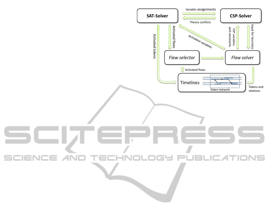
Figure 1: J-TRE architecture. The SAT solver controls most
of the search aspects notifying the CSP solver of variable
assignments. The planner collects active flaws, selects one
of them and solves it by adding new relations among tokens
and/or new tokens into the token network. The planning
process will result in a partially active token network with
no active flaws.
SAT and CSP solving (see Figure 1).
As a starting point we have used an implementa-
tion of the known MiniSAT solver (Een and Sorens-
son, 2003) modified to endow it with capabilities for
handling both preferences (Di Rosa et al., 2010) and
dynamic addition of variables and clauses.
A second step has been to produce a backtrack-
able AC-3 algorithm (one of the most often used al-
gorithms by simple constraint satisfaction solvers).
We consider a constraint satisfaction problem as a di-
rected graph (Dechter, 2003) with nodes representing
variables of the problem and arcs between variables
representing constraints. Special attention is given to
efficiency of basic reasoning. The worst-case time
complexity of AC-3 algorithm is O
e· d
3
where e
is the number of arcs and d is the size of the largest
variable domain. It is worth underscoring that two key
complexity factors here are the need to tackle huge
domains (e.g., [0, +inf] is a common domain for tem-
poral arguments) and possible presence of cyclic net-
works. For each constraint addition to the CSP, we
have limited the number of possible updates of each
variable to the number of constraints of the CSP. Ex-
ceeding this limit would obviously determines the ex-
istence of a cycle that incrementally empties the do-
main of some variable involved in the cycle itself re-
sulting in an inconsistent CSP. This fact allowed us to
move worst-case time complexity of our AC-3 algo-
rithm to O(e· min(e, d)) removing the discouraging
domain size from time complexity.
Interplay between SAT and CSP. Any CSP con-
straint has a correspondent SAT variable that “acti-
vates” it. As soon as an activation variable becomes
NEW REASONING FOR TIMELINE BASED PLANNING - An Introduction to J-TRE and its Features
147

true in the SAT its correspondent constraint is dynam-
ically added to the CSP and propagation is triggered
with AC-3. The interplay works also the other way
around: if a SAT variable goes from true to non as-
signed (when the SAT solver is either backtracking or
backjumping) then the corresponding constraint in the
CSP is “deactivated” retracting it from the dynamic
CSP that again is propagated to the previous situa-
tion. It is worth observing that because the SAT solver
manipulate variables according to a Last In First Out
strategy this facilitates efficiency of retraction in the
correspondent dynamic CSP (before propagation a
cashing mechanism of domains serves the future re-
tractions). Furthermore, not all the SAT variables
have a correspondent constraint. Those that are free
from this connection are used to model the causality
in the planning problem.
When the CSP propagation fails we have a theory
conflict. The SAT solver is consistent but the corre-
spondent theory represented by the CSP (the set of ac-
tive constraints) is not. Similarly to the lazy approach
in SMT we add the information on the theory failure
in the SAT representation by adding the negation of
the conjunction of active constraints hence avoiding
that the SAT solver reselect the same state later on.
It is worth saying that the negation of a conjunc-
tion of literals can be transformed in a disjunction
of negation by using De Morgan. In the SAT rea-
soner this new clause is considered as a new “conflict
clause” from which a no-good is generated and added
the the representation before a backtracking step.
In addition, by giving preference for false val-
ues to each SAT variable allows us to minimize the
number of active elements in the token network and,
consequently, the number of active CSP constraints.
Our extended CSP solver can now handle disjunctive
CSPs and domain causality through the SAT problem.
If the SAT problem would become unsatisfiable then
our extended CSP problem would have no solutions.
Using the Hybrid Reasoning Engine for Time-
line based Planning. We now describe how the
SAT/CSP combination is used to model the timeline-
based approach to planning. Each token, each rela-
tions (and also each of the flaws introduced later) has
an “activation variable”. The glue among these vari-
ables is given by the domain causality. For example,
the activation variable of a token can logically imply
the activation variable of the relation that represent
the duration of the same token. When the activation
variable becomes true, the SAT solver naturally prop-
agate truth also to the activation variable of the rela-
tion. Hence the whole “causality pattern” is added to
the correspondent dynamic CSP.
The very hard part of the work has been the
representation of quantitative Allen relations (Allen,
1983) with quantitative modificators. For ex-
ample we need to represent bef ore(i, j, min, max)
that forces interval i to be be fore interval j
with a distance [min, max] between i.e and j.s, or
during(i, j, min
1
, max
1
, min
2
, max
2
), forcing interval
i to be during interval j with a distance [min
1
, max
1
]
between j.s and i.s and a distance [min
2
, max
2
] be-
tween i.e and j.e. As a first ingredient we need a sim-
ple temporal constraint (Dechter, 2003) between two
time points. The constraint has to propagate accord-
ing to the bounds on distances min ≤ x
1
− x
0
≤ max
where x
0
and x
1
are the starting and ending point of
the constraint and min and max are the limitations
the two points must be bounded at. Having this ex-
pressivity allows as to impose a duration constraint
[l, u] for a token t having starting point t.s and end-
ing point t.e we have to add the simple temporal con-
straint l ≤ t.e− t.s ≤ u.
An exhaustive enumeration and description of all
the relation implemented by our planning system is
outside the scope of this paper. We just provide here
the underlying idea by explaining of howthe overlaps
constraint has been managed. Given a token t
0
having
starting point t
0
.s and ending point t
0
.e and a token
t
1
having starting point t
1
.s and ending point t
1
.e, the
overlaps constraint is defined through a simple tem-
poral constraint between t
0
.e and t
1
.s (let us associate
this to the activation variable x
0
), a simple tempo-
ral constraint between t
1
.s and t
0
.e (x
1
) and a sim-
ple temporal constraint between t
0
.e and t
1
.e (x
2
). In
creating the overlaps constraint we assign it an ac-
tivation variable x
overlaps
and assign the three sim-
ple temporal constraints to their SAT variables x
0
, x
1
and x
2
. Finally we add the clauses
¬x
overlaps
, x
0
,
¬x
overlaps
, x
1
and
¬x
overlaps
, x
2
to the SAT prob-
lem. It is worth underscoring that the false preference
of the SAT solver instantiates the activated temporal
constraints if and only if x
overlaps
becomes true.
Once defined all relations allowed by the system,
it is relatively straightforward to combine them in a
logical way. For example, if we do not want two to-
kens t
0
and t
1
to overlap, we can create two relations
before(t
0
,t
1
, 0, +inf) and a fter(t
0
,t
1
, 0, +inf), hav-
ing activation variable x
b
and x
a
, and add the clause
(x
b
, x
a
) to our extended CSP solver. Although not
necessary (indeed, the CSP propagation and conflict
analysis will generate it as a no-good sooner or later),
we can also add the clause (¬x
b
, ¬x
a
) that will avoid
useless propagation of CSP constraints.
By embedding both disjunctions and causal rela-
tions in our CSP solver we are able to hide search
space to higher level modules favoring the high-
ICAART 2012 - International Conference on Agents and Artificial Intelligence
148

light of higher level search aspects as planning and
scheduling heuristics.
Conflict Analysis: No-good Learning and Back-
jumping. Conflict-driven clause learning has been
first described in (Marques-Silva et al., 1996) and
is commonly considered a key advantage of SAT-
technology in the last decade. We will describe how
it works and the use we do of it through an example
adapted from (Een and Sorensson, 2003).
Assume we have three CSP constraints associ-
ated to variables x
0
, x
1
and x
2
. Our constraints, to-
gether, make the CSP problem inconsistent so the
clause (¬x
0
, ¬x
1
, ¬x
2
) represents our conflict to ana-
lyze. We call x
0
∧x
1
∧x
2
the reason set of the conflict.
Now x
0
is true because x
0
was propagated from some
clause. That clause is asked the reason for propagat-
ing x
0
and it responds with another conjunction of lit-
erals, say x
3
∧ x
4
. These are the variable assignments
that implied x
0
. The clause may in fact have been
(x
0
, ¬x
3
, ¬x
4
). From this little analysis we know that
x
3
∧ x
4
∧ x
1
∧ x
2
must lead to a conflict. We prohibit
this conflict by adding the clause (¬x
3
, ¬x
4
, ¬x
1
, ¬x
2
)
to the SAT problem. This would be an example of
learnt conflict clause.
Analyzing further all literals and their reason sets
would lead to different learning schemas however the
“First Unique Implication Point” (First UIP) has been
chosen for its effectiveness (Zhang et al., 2001). The
underlying idea is quite simple: in a breadth-first
manner, continue to expand literals of the current de-
cision level until there is just one left. As in Min-
iSAT, the analysis also returns the lowest decision
level for which the conflict clause is unit allowing
non-chronological backtracking.
Notice that, in our case, learnt clauses would rep-
resent information such as: “two constraints cannot
be in the same state” which, broadly speaking, is
a much more useful information with respect to a
generic “current state is inconsistent”.
Clause Database Simplification. Common SAT
solvers often benefit from clause database simplifica-
tion reducing the size of the problem. The procedure
has to check the status of all literals of all clauses in
order to apply simplification resulting in a quite ex-
pensive procedure.
First of all, SAT clauses simplification is only
available at top-level. After an initial propagation,
each SAT clause may simplify its representation or
state that the clause is satisfied under the current as-
signment and can be removed. Let’s assume we have
the clauses (x
0
), (¬x
0
, x
1
, x
2
, x
3
) and (x
0
, x
4
, x
5
). Ini-
tial propagation would assign true value to variable x
0
and clause simplification would reduce second clause
to (x
1
, x
2
, x
3
) and remove third clause.
In our application to planning, clause database
simplification leads to an interesting behavior that we
would like to highlight. This procedure, basically,
hides elements of the token network that, for sure, are
true (or false) highlighting elements of the token net-
work that are still uncertain. This latter set represents
the “real planning problem” as it requires an effective
search phase (with possible backtracking) to work on.
4 ENSURING TIMELINE
CONSISTENCY: DETECTING
FLAWS AND SOLVING THEM
Common timeline based planners reach a solution
state by applying an iterative refinement procedure.
If we call flaw every possible inconsistency of the to-
ken network, the role of the planner can be reduced
to flaws identification in the current token network
and their consequent resolution. The planning pro-
cess goes on until a consistent (no flaws) token net-
work is found. The general idea is simply to have
a set of flaws, pick one with some selection strategy
and solve it with some resolution strategy (this is rep-
resented in Figure 1 by the blocks Flaw Selector and
Flaw Solver). There are basically two kinds of pos-
sible flaws: goal flaws and timeline inconsistency
flaws.
Once defined how to represent information, we
have to understand how the planner can identify as-
pects of the current token network and fix them in or-
der to reach the desired token network that includes
the set of goals. We do not introduce any innovation
on this phase, we will rather show how our proposal
can easily be applied to common approaches. First of
all, as in the case of tokens and relations, we assign
each flaw an activation variable that can be used to
control flaw’s activation status. As always, the false
preference for SAT variables will guarantee us that
the flaw will be disabled unless it has strictly to be
activated.
First thing we do is to generate the initial token
network. Initial fact tokens as well as relations must
be present so we add a unary clause for each of them
forcing the truth of their activation variables. We do
the same for goal tokens as they have to be justified
in order for the problem to be solved but, for each of
them, we enqueue a goal flaw assigning it the same
activation variable of the relative token. This means
that the goal flaw will be active only if the relative to-
ken’s activation variable is true.
NEW REASONING FOR TIMELINE BASED PLANNING - An Introduction to J-TRE and its Features
149

In the following, we will use the symbol S to indi-
cate the conjunction of all activation variable of both
tokens and relations that in current state are active. In
particular, exploiting De Morgan laws, we will use the
symbol ¬S to indicate the disjunction of negations of
the literals of S. Being a disjunction of literals, with a
little extension of terminology, we will use ¬S inside
clauses.
4.1 Goal Flaws
For what concerns goal flaws, we have two possible
resolution strategies: unification and compatibility ex-
pansion.
Unification is only applicable to tokens that have
the same proposition. For the sake of compactness,
we have introduced a new CSP constraint, that we call
“multi-equals”, defined as follows: given two sets of
CSP variables [x
0
, . . . , x
n
] and [y
0
, . . . , y
n
], the multi-
equals constraint is satisfied iff [x
0
= y
0
, . . . , x
n
= y
n
].
Exploiting our multi-equals constraint we assign a
SAT variable u
0
, . . . , u
i
, . . . , u
n
, for each of the n to-
kens (eventually none if unification is clearly infea-
sible) on the same timeline having the same propo-
sition, to a multi-equals constraint that will ensure
equality between goal token’s arguments and target
token’s arguments. Whenever a variable u
i
becomes
true, the token is forced to unify with the correspon-
dent token. We also create a new SAT variable c that
will force compatibility application. The flaw solver
will then add the resolution clause (¬ f, u
0
, . . . , u
n
, c)
and will apply the compatibility as an implication by
the compatibility application variable c managing tar-
get tokens as new goal flaws (sub-goaling).
Let us assume that we have a compatibil-
ity associated to predicate P() such that P() ⇒
(q : Q() ∧ during(this, q)) and a goal token with ac-
tivation variable g and proposition P() (meaning that
I want to achieve g on the solution timeline). We first
create a token with activation variable q and a propo-
sition Q(), then we create a relation during with ac-
tivation variable r between token with activation vari-
able g and token with activation variable q, finally we
add clauses (¬c, q) and (¬c, r).
Because unification does not lead to further com-
patibilities application, we add preference constraints
to the SAT problem in order to prefer unifications to
compatibility application. Thus we have ∀i = 1. . . n :
c ≺ u
i
. Notice that, having preferences for false val-
ues, we have inverted preference order on variable se-
lection. In so doing, we are stating that we want com-
patibility variable at false before unification variable
is at false.
Must-expand and Must-unify Operators for Goal
Flaws. Some timeline based planners make use of
must-expand and must-unify domain dependent oper-
ators applied to goal flaws in order to force the planner
to behave in a desired manner, namely pruning search
space. The idea is simply that must-expand goal flaws
cannot unify while must-unify goal flaws cannot ap-
ply their compatibility.
The must-expand operator can be managed sim-
ply adding the resolution clause without the unifica-
tion variables (¬ f, c). The must-unify operator is
more tricky because we first have to add the resolu-
tion clause with the negation of current state and with-
out the compatibility variable (¬ f, ¬S, u
0
, . . . , u
n
),
and then we have to create another flaw with ac-
tivation variable f
0
and add an activation clause
(¬ f, u
0
, . . . , u
n
, f
0
). If none of such unifications is
applicable, first clause will make current state un-
available while second clause will activate the derived
flaw. Both cases are implied by the activation of the
original flaw.
4.2 Timeline Inconsistencies and the
Use of Schedulers
Once the overall solving procedure has reached a sta-
ble state (that is there is no active goal flaw), for
each timeline is called a make-consistent procedure
that, dependent on the timeline itself, removes any
further inconsistencies from the timeline through a
scheduling procedure. This is a technique, intro-
duced in (Fratini et al., 2008), that observes time-
lines as resources over time and removes contentions
peaks over their continuous representation. We will
not discuss how the scheduling flaws are identified
(aka contention peaks) here and refer the reader to
(Cesta et al., 2002) for details on reusable resources,
used to model the RCPSP/max problem, and to (Si-
monis and Cornelissens, 1995) on how to manage
producer/consumer constraints, required in replenish-
able resource timelines, through a resource contention
greedy solver.
Once we have identified a Minimal Conflict Set
(MCS) of tokens that have to be scheduled on a time-
line, we simply enqueue it as a common flaw and
assign it an activation variable s. This variable will
be implied by current state so the activation clause
is (¬S, s). The resolution of the scheduling flaw will
simply add a disjunction on the ordering of the tokens
adding proper constraints.
For example, we have an MCS with activation
variable s composed by two tokens t
0
and t
1
. The
flow resolution procedure will generate two relations
t
0
≺ t
1
and t
1
≺ t
0
associating them two activation
ICAART 2012 - International Conference on Agents and Artificial Intelligence
150

variables b and a. Finally, the clause (¬s, b, a) is
added to the SAT problem. Once again, the clause
(¬b, ¬a) can also be added to improve performances.
It is worth noting that, at present, we are not inter-
ested in obtaining an optimal solution for the schedul-
ing problem minimizing the overall make-span but we
are rather looking for a solution that just makes the
timeline consistent. In case there is the need of op-
timizing the make-span in the scheduling phase, we
can always rebuild the all-pair-shortest-path problem
(as common timeline based planners currently do for
any search space state) and use it to build heuristics
assigning ordering preferences on the activation vari-
ables of the relations of the MCS (as always, taking
into account the false preference for SAT variables).
In this case the system would still provide complete-
ness of the search as well as back-jumping features
and even more.
5 THE J-TRE ARCHITECTURE
In order to enable a comparison with other timeline
based planners, we have completely implemented the
architecture in Figure 1 as a Java program. Addi-
tionally, we have defined an XML-based modeling
language, called eXtended Domain Definition Lan-
guage (XDDL), that allows us to create domains and
problems for the planner. Most of the search is de-
manded to the SAT solver that notifies the CSP solver
of variable assignments. The CSP solver, in turn,
propagates activated constraints (or backtracks) and,
in case propagation fails, a conflict clause is added to
the SAT problem. The planner collects active flaws,
selects one of them according to a selection strategy
and solves it through a resolution strategy by adding
new relations among tokens and/or new tokens into
the token network.
While, in our system, there is almost no differ-
ence in which flaw is solved first (as far as we ignore
efficiency aspects) because they all have to be solved
sooner or later, there could be serious troubles in how
they are solved, especially in case of cyclic problems.
Consider, for example, a two predicates state vari-
able having At (l, s, e) and GoingTo(l, s, e) as allowed
values. Moreover there is a compatibility for predi-
cate At to start at 0 or to be met by a GoingTo pred-
icate with same location. Finally, a compatibility for
predicate GoingTo to be met by a predicate At. We
have an initial state with a token At (l
0
, 0, [1, + inf])
and a goal At(l
3
, [0, +inf], [1, +inf]). The planner
has to apply compatibility for goal token produc-
ing a sub-goal GoingTo(l
3
, [0, + inf], [1, +inf]) than
another sub-goal At (l, [0, +inf], [1, + inf]) that can
unify with first token or apply another compatibility
resulting in another GoingTo(l, [0, +inf], [1, + inf])
possibly leading to an infinite loop planning about
the agent going walking around. In short, although
scheduling search space, however exponential, is al-
ways finite, it can be the case that compatibility appli-
cation space is infinite.
Although a crafty strategy does not exist yet (ex-
ception made for some work by Bernardini (Bernar-
dini and Smith, 2007) that basically prefers smallest
sub-goaling to greater ones) we can exploit SAT pref-
erences to guide the search at domain definition level.
Another simple thing we can do to avoid taking the
wrong path is to give preferences according to the
depth of the search tree leading to a sort of breadth-
first search. However, possible solutions to this prob-
lem still need to be investigated.
6 A PRELIMINARY EVALUATION
In this section we describe a preliminary evaluation
based on a competitive evaluation with respect to the
version 1.99 of the OMPS planner, an evolution of the
work described in (Fratini et al., 2008).
To perform the comparison we have created two
“simple-to-describe” domains that require causal rea-
soning over time. We have chosen these domains
for their requirement of both planning and scheduling
features as well as for their simplicity.
Because of the randomness of resolution algo-
rithms, results were obtained by averaging the exe-
cution time of 10 run for each problem. We did not
use any domain dependent operators nor domain de-
pendent heuristics in none of the planners with the
intent of comparing pure approaches to search. Both
planners, indeed, can be easily speeded up through
domain dependent operators – as done for example
in the very last OMPS version used in (Fratini et al.,
2011). Finally, we set the OMPS planner to apply the
depth first resolution strategy, which seems to be on
average the most promising resolution strategy among
those available.
The Skilift Domain. This domain models peo-
ple flow while taking a skilift in a skiing sta-
tion. The domain uses a state variable with
two allowed values: takeSkilift (p, s, e), modelling
a person p taking the skilift and unused (s,e).
Each modeled person has his own timeline repre-
senting his position through downstream(s, e) and
upstream(s, e) predicates. Furthermore, there is a
compatibility for predicate upstream to have a du-
ration of [10, + inf] and to be met by a takeSkilift
NEW REASONING FOR TIMELINE BASED PLANNING - An Introduction to J-TRE and its Features
151
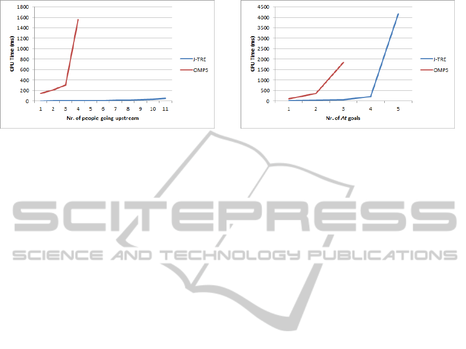
Figure 2: The skilift domain: J-TRE results compared with
OMPS 1.99 planner. The number of people that go upstream
on the abscissas and planning resolution procedure execu-
tion time on the ordinates.
predicate with parameter equal to the person id
and a relation that meets a predicate downstream
with the takeSkilift predicate. Finally, predicate
takeSkilift (p, s, e) has a compatibility requiring a du-
ration [50, + inf]. Initial state is constituted by a single
token downstream(x, 0, [1, +inf]) with x the id of the
person and a goal upstream([0, + inf], [1, + inf]). We
scale the problem by adding more people. Figure 2
shows execution time (in milliseconds) of our bench-
mark problem with increasing number of people go-
ing upstream on the horizontal axis. OMPS planner
requires, on average, too much time already at fourth
instance of problems.
The Walkin’ Robot Domain. The second domain
introduces a slightly more difficult problem for time-
line based planners. We have a single state vari-
able with only two allowed values: At (x, y, s, e) and
GoingTo(x, y, s, e). There is a compatibility for pred-
icate At to have a duration of [10, +inf] and to start
at 0 or to be met by a GoingTo predicate with
same coordinates. Finally, a compatibility for pred-
icate GoingTo to have a duration of [10, +inf] and
to be met by a predicate At. While initial state
is constituted by a single token At (0, 0, 0, [1, + inf]),
we will incrementally add different goals of type
At(x
g
, y
g
, [0, +inf], [1, + inf]) and will let the planner
to solve the growing problem.
Figure 3 shows execution time (in milliseconds)
of our benchmark problem (having the number of At
goals on the abscissas). Although this problem may
seem easy (a similar problem, deprived of time, could
be solved in no time by classical planner), indeed
it requires quite hard planning and scheduling fea-
tures forcing the planner to chose an ordering between
goals scheduling At tokens as well as GoingTo ones.
The planner has to continuously chose the tokens with
whom to unify and has to manage disjunctions on the
Figure 3: The walkin’ robot domain: J-TRE results com-
pared with OMPS 1.99 planner. The number of visited lo-
cations on the abscissas and planning resolution procedure
execution time on the ordinates.
definition of compatibilities.
Despite complexity, J-TRE outperforms OMPS
but encounters difficulties in scaling up at the sixth in-
stance of the problem. This second type of domains,
requiring harder scheduling skills, identify a direction
of study for future developments.
7 CONCLUSIONS
Most common AI applications, as planning and
scheduling, require a high degree of parallelism in
order to consider simultaneously different available
evolutions. Current state-of-the-art SAT-solvers can
solve really complex problems in small time thanks
to no-goodlearning and non-chronologicalbacktrack-
ing mixed with efficient propagation procedures and
dynamic variable ordering (Moskewicz et al., 2001).
Finally, adding preferences to SAT solving enables us
to cope with qualitative aspects of the obtained solu-
tions.
An advantage of our proposal is the possibility
of fast movements from one state to another taking
benefit of similarities of different nodes of the search
space. From a technical point of view, the planner
implementation is significantly simplified (e.g., we
created a new planner with a somehow limited time
effort) thanks to the implicit search space and, fur-
thermore, in the direct correspondence between con-
cepts and solvers. This will allow us to concentrate on
higher level aspects of search as domain independent
heuristics.
Nevertheless, this is a first feasibility study in this
research direction and a lot of work remains to be
done. For what concerns our XDDL language, we
have to increase its modularity (as in NDDL (Jons-
son et al., 2000)) in order to allow the generation of
complex domains by end users. Also, the definition of
ICAART 2012 - International Conference on Agents and Artificial Intelligence
152

domain dependent heuristics will be subject of future
studies.
Loss of information due to our AC-3 implemen-
tation, that does not take care of distances between
time points can be extracted as well with already
known techniques having available active tokens and
relations. This information could be used to gen-
erate heuristics providing preferences on choices on
the search space. The hypothesis of using our AC-
3 algorithm to solve an all-pair-shortest-path has not
been investigated yet, although we think that using
already known techniques is a preferred choice. This
hypothesis, indeed, would provide useful information
for heuristics by slightly changing the architecture at
the cost of having an extra CSP variable for each cou-
ple of real CSP variable used by the planner in order
to maintain the distance between them. Cost that, in-
tuitively, will be significantly high.
Execution time would definitely benefit of a
tighter integration of SAT and CSP solvers coming
from most recent SMT techniques. CSP constraints,
for example, could be buffered and propagated all at
once after SAT propagation is finished. Finally, dis-
junctive qualitative temporal reasoning could be used
as a background infrastructure in order to add more
constraints to the SAT solver avoiding expensive CSP
propagation.
ACKNOWLEDGEMENTS
Authors are partially supported by EU under the PAN-
DORA project (Contract FP7.225387) and by MIUR
under the PRIN project 20089M932N (funds 2008).
Authors would like to thank Simone Fratini for joint
work on timeline-based planning and Andrea Orlan-
dini for comments to a previous version of the paper.
REFERENCES
Allen, J. F. (1983). Maintaining Knowledge about Temporal
Intervals. Commun. ACM, 26(11):832–843.
Bedrax-Weiss, T., McGann, C., and Ramakrishnan, S.
(2003). Formalizing Resources for Planning. In Pro-
ceedings of the Workshop on Planning Domain De-
scription Language at ICAPS-03, pages 7–14.
Bernardini, S. and Smith, D. (2007). Developing domain-
independent search control for EUROPA2. In Pro-
ceedings of the Workshop on Heuristics for Domain-
independent Planning at ICAPS-07.
Cesta, A., Oddi, A., and Smith, S. F. (2002). A Constraint-
based Method for Project Scheduling with Time Win-
dows. Journal of Heuristics, 8(1):109–136.
Dechter, R. (2003). Constraint Processing. Morgan Kauf-
mann.
Di Rosa, E., Giunchiglia, E., and Maratea, M. (2010). Solv-
ing Satisfiability Problems with Preferences. Con-
straints, 15(4):485–515.
Een, N. and Sorensson, N. (2003). An Extensible SAT-
Solver. In Giunchiglia, E. and Tacchella, A., editors,
SAT, volume 2919 of Lecture Notes in Computer Sci-
ence, pages 502–518. Springer.
Erol, K., Hendler, J., and Nau, D. S. (1994). HTN Planning:
Complexity and Expressivity. In AAAI-94. Proceed-
ings of the Twelfth National Conference on Artificial
Intelligence.
Fox, M. and Long, D. (2003). PDDL2.1: An Exten-
sion to PDDL for Expressing Temporal Planning Do-
mains. Journal of Artificial Intelligence Research,
20:61–124.
Frank, J. and Jonsson, A. (2003). Constraint-Based At-
tribute and Interval Planning. Constraints, 8(4):339–
364.
Fratini, S., Cesta, A., Orlandini, A., Rasconi, R., and
De Benedictis, R. (2011). APSI-based Deliberation in
Goal Oriented Autonomous Controllers. In Proc. of
11th ESA Symposium on Advanced Space Technolo-
gies in Robotics and Automation (ASTRA).
Fratini, S., Pecora, F., and Cesta, A. (2008). Unifying Plan-
ning and Scheduling as Timelines in a Component-
Based Perspective. Archives of Control Sciences,
18(2):231–271.
Ghallab, M. and Laruelle, H. (1994). Representation and
Control in IxTeT, a Temporal Planner. In AIPS-94.
Proceedings of the 2nd Int. Conf. on AI Planning and
Scheduling, pages 61–67.
Jonsson, A., Morris, P., Muscettola, N., Rajan, K., and
Smith, B. (2000). Planning in Interplanetary Space:
Theory and Practice. In AIPS-00. Proceedings of the
Fifth Int. Conf. on AI Planning and Scheduling.
Marques-Silva, J. P., Silva, J. P. M., Sakallah, K. A., and
Sakallah, K. A. (1996). GRASP - A New Search Al-
gorithm for Satisfiability. In Proceedings of the In-
ternational Conference on Computer-Aided Design,
pages 220–227.
Moskewicz, M. W., Madigan, C. F., Zhao, Y., Zhang, L.,
and Malik, S. (2001). Chaff: Engineering an Efficient
SAT Solver. In Proceedings of the 38th Annual Design
Automation Conference, pages 530–535.
Muscettola, N. (1994). HSTS: Integrating Planning and
Scheduling. In Zweben, M. and Fox, M.S., editor,
Intelligent Scheduling. Morgan Kauffmann.
Sebastiani, R. (2007). Lazy Satisability Modulo Theories.
JSAT, 3(3-4):141–224.
Simonis, H. and Cornelissens, T. (1995). Modelling Pro-
ducer/Consumer Constraints. In CP-95. Proceedings
of the First International Conference on Principles
and Practice of Constraint Programming, pages 449–
462, London, UK. Springer-Verlag.
Smith, D., Frank, J., and Jonsson, A. (2000). Bridging the
Gap Between Planning and Scheduling. Knowledge
Engineering Review, 15(1):47–83.
Zhang, L., Madigan, C. F., Moskewicz, M. H., and Ma-
lik, S. (2001). Efficient Conflict Driven Learning in
a Boolean Satisfiability Solver. In ICCAD ’01. Pro-
ceedings of the 2001 IEEE/ACM international confer-
ence on Computer-aided design, pages 279–285, Pis-
cataway, NJ, USA. IEEE Press.
NEW REASONING FOR TIMELINE BASED PLANNING - An Introduction to J-TRE and its Features
153
