
A TRACTABLE FORMALISM FOR COMBINING RECTANGULAR
CARDINAL RELATIONS WITH METRIC CONSTRAINTS
Angelo Montanari
1
, Isabel Navarrete
2
, Guido Sciavicco
2
and Alberto Tonon
1
1
Department of Mathematics and Computer Science, University of Udine, Udine, Italy
2
Department of Information Engineering, University of Murcia, Murcia, Spain
Keywords:
Qualitative spatial reasoning, Quantitative spatial reasoning, Cardinal direction relations, Constraint satisfac-
tion problems.
Abstract:
Knowledge representation and reasoning in real-world applications often require to integrate multiple aspects
of space. In this paper, we focus our attention on the so-called Rectangular Cardinal Direction calculus for
qualitative spatial reasoning on cardinal relations between rectangles whose sides are aligned to the axes of the
plane. We first show how to extend a tractable fragment of such a calculus with metric constraints preserving
tractability. Then, we illustrate how the resulting formalism makes it possible to represent available knowledge
on directional relations between rectangles and to derive additional information about them, as well as to
deal with metric constraints on the height/width of a rectangle or on the vertical/horizontal distance between
rectangles.
1 INTRODUCTION
Qualitative spatial representation and reasoning play
an important role in various areas of computer sci-
ence such as, for instance, geographic information
systems, spatial databases, document analysis, lay-
out design, and image retrieval. Different aspects of
space, such as direction, topology, size, and distance,
which must be dealt with in a coherent way in many
real-world applications, have been modeled by differ-
ent formal systems (Broxvall, 2002; Condotta, 2000;
Gerevini and Renz, 2002; Liu et al., 2009) (see (Cohn
and Hazarika, 2001) for a survey). For practical rea-
sons, a bidimensional space is commonly assumed,
and spatial entities are represented by points, boxes,
or polygons with a variety of shapes, depending on
the required level of detail.
Information about spatial configurations is usually
specified by constraint networks describing the al-
lowed binary relations between pairs of spatial vari-
ables. The central problem in qualitative reasoning is
consistency checking, which is the problem of decid-
ing whether or not a network has a solution, that is,
the problem of establishing whether or not there ex-
ists an assignment of domain values to variables that
satisfies all constraints.
Cardinal relations are directional relationships
that allow one to specify how spatial objects are
placed relative to one another either by making use
of a fixed reference system, e.g., to say that an object
is to the “north” or “southwest” of another one in a ge-
ographic space, or, alternatively, by exploiting direc-
tions as “above” or “below and left” in a local space.
Cardinal relations are of particular interest for geo-
graphic information systems, spatial databases, and
image databases (Frank, 1996; Goyal, 2000; Papadias
and Theodoridis, 1997; Skiadopoulos et al., 2005).
The most expressive formalism with cardinal rela-
tions between extended spatial objects is the Cardi-
nal Direction calculus, CD-calculus for short (Goyal
and Egenhofer, 2000; Liu et al., 2010; Skiadopou-
los and Koubarakis, 2005). The consistency problem
for the CD-calculus is NP-complete, and no tractable
fragment of it has been identified so far, with the
only exceptionof the fragment obtained by forbidding
disjunctive relations (Skiadopoulos and Koubarakis,
2005). Such a restriction is a serious limitation when
we have to deal with incomplete or indefinite infor-
mation in spatial applications.
In (Navarrete and Sciavicco, 2006), the au-
thors introduce a restricted version of the CD-
calculus called Rectangular Cardinal Direction cal-
culus (RCD-calculus), where cardinal relations are
defined only between rectangles whose sides are par-
allel to the axes of the Euclidean plane. Rectangles
of this type (boxes) can be seen as minimum bound-
154
Montanari A., Navarrete I., Sciavicco G. and Tonon A..
A TRACTABLE FORMALISM FOR COMBINING RECTANGULAR CARDINAL RELATIONS WITH METRIC CONSTRAINTS.
DOI: 10.5220/0003747901540163
In Proceedings of the 4th International Conference on Agents and Artificial Intelligence (ICAART-2012), pages 154-163
ISBN: 978-989-8425-95-9
Copyright
c
2012 SCITEPRESS (Science and Technology Publications, Lda.)

ing rectangles (MBRs) that enclose plane regions (the
actual spatial objects). MBRs have been widely used
in spatial databases (El-Geresy and Abdelmoty, 2001;
Papadias and Theodoridis, 1997), in web-document
analysis (Gatterbauer and Bohunsky, 2006), and in
2D-layout design, e.g., in architecture (Baykan and
Fox, 1997). On the one hand, approximating regions
by rectangles implies a loss of accuracy in the rep-
resentation of the relative direction between regions;
on the other hand, reasoning tasks become more effi-
cient.
The RCD-calculus has a strong connection with the
Rectangle Algebra (RA) (Balbiani et al., 1998), which
can be viewed as a bidimensional extension of Inter-
val Algebra (IA), the well-knowntemporal formalism
for dealing with qualitative binary relations between
time intervals (Allen, 1983). A tractable fragment
of the RCD-calculus, named convex RCD-calculus,
has been identified by Navarrete et al. in (Navarrete
et al., 2011). It includes all basic relations and a large
number of disjunctive relations, making it possible to
represent and reason about indefinite information ef-
ficiently.
This paper aims at adding metric features to for-
malisms for qualitative spatial reasoning. Metric con-
straints between points over a dense linear order have
been dealt with by the Temporal Constraint Satis-
faction Problem formalism (TCSP) (Dechter et al.,
1991). In such a formalism, one can constrain the dis-
tance between a pair of points to belong to a given set
of intervals. If each constraint consists of one inter-
val only, we get a tractable fragment of TCSP, called
Simple Temporal Problem formalism (STP).
In the following, we propose a metric extension to
the convex RCD-calculus that allows one to repre-
sent available knowledge on directional relations be-
tween rectangles and to derive additional informa-
tion about them, as well as to deal with metric con-
straints on the height/width of a rectangle or on the
vertical/horizontal distance between rectangles. We
will show that the resulting formalism is expressive
enough to capture various scenarios of practical inter-
est and still computationally affordable.
The rest of the paper is organized as follows.
In Section 2, we provide background knowledge on
qualitative calculi and we shortly recall Interval Al-
gebra and Rectangle Algebra. In Section 3, we intro-
duce RCD-calculus and its convex fragment. In Sec-
tion 4, we extend the convex RCD-calculus with met-
ric constraints, and we devise a sound and complete
polynomial algorithm for consistency checking. We
conclude the section with a simple application exam-
ple. Conclusions provide an assessment of the work
and outline future research directions.
Figure 1: Basic relations of the Interval Algebra.
2 PRELIMINARIES
In this section, we introduce basic notions and termi-
nology.
Temporal knowledge, as well as spatial knowl-
edge, is commonly represented in a qualitative cal-
culus by means of a qualitative network consisting
of a complete constraint-labeled digraph N = (V,C),
where V = {v
1
, . . . , v
n
} is a finite set of variables, in-
terpreted over an infinite domain D, and the labeled
edges in C specify the constraints describing qual-
itative spatial or temporal configurations. An edge
from v
i
to v
j
labeled with R corresponds to the con-
straint v
i
Rv
j
, where R denotes a binary relation over
D which restricts the possible values for the pair of
variables (v
i
, v
j
). The full set of relations of the cal-
culus is usually taken as the powerset 2
B
, where B
is a finite set of binary basic relations that forms a
partition of D × D. Thus, a relation R
ij
∈ 2
B
is of
the form R = {r
1
, . . . , r
m
}, where each r
i
is a basic
relation, and R represents the union of the basic rela-
tions it contains. If m = 1, we call R a basic relation;
otherwise, we call it a disjunctive relation. A special
case of disjunctive relation is the universal relation,
denoted by ‘?’, which contains all the basic relations.
A basic constraint v
i
{r}v
j
expresses definite knowl-
edge about the values that the two variables v
i
, v
j
can
take, while a disjunctive constraint v
i
{r
1
, . . . , r
m
}v
j
expresses indefinite or imprecise knowledge about
these values. In particular, the universal constraint
v
i
?v
j
states that the relation between v
i
an v
j
is to-
tally unknown. From a logical point of view, a dis-
junctive constraint v
i
{r
1
, . . . , r
m
}v
j
can be viewed as
the logical disjunction v
i
{r
1
} v
j
∨ ·· · ∨ v
i
{r
m
} v
j
.
An instantiation (or interpretation) of the con-
straints of a qualitative network N is a mapping ι rep-
resenting an assignment of domain values to the vari-
ables of N. A constraint v
i
Rv
j
is said to be satisfied
by an instantiation ι if the pair (ι(v
i
), ι(v
j
)) belongs
to the binary relation represented by R. A consistent
A TRACTABLE FORMALISM FOR COMBINING RECTANGULAR CARDINAL RELATIONS WITH METRIC
CONSTRAINTS
155

instantiation, or solution, of a network is an assign-
ment of domain values to variables satisfying all the
constraints. If such a solution exists, then the network
is consistent, otherwise it is inconsistent.
The main reasoning task in qualitative reasoning
is consistency checking, which amounts to deciding if
a network is consistent. If all relations are considered,
consistency checking is usually NP-hard. Hence,
finding subsets of 2
B
for which consistency check-
ing turns out to be polynomial (tractable subsets) is
an important issue to address. Another common task
in qualitative reasoning is computing the unique mini-
mal network equivalentto a given one by determining,
for each pair of variables, the strongest relation (min-
imal relation) entailed by the constraints of the net-
work. It can be easily shown that each basic relation
in a minimal network is feasible, i.e., it participates in
some solution of the network.
To deal with these tasks, constraint propagation
techniques are usually exploited. The most promi-
nent method for constraint propagation is the path-
consistency algorithm, PC-algorithm for short (Mack-
worth, 1977). Such an algorithm refines relations
by successively applying the operation R
ij
← R
ij
∩
(R
ik
◦ R
kj
) for every triple of variables (v
i
, v
k
, v
j
), un-
til a stable network is reached, where R
ij
, R
ik
, R
kj
are the relations constraining the pair of variables
(v
i
, v
j
), (v
i
, v
k
), (v
k
, v
j
), respectively (◦ stands for the
composition of relations). If the empty relation is ob-
tained during the process, then the input network is in-
consistent; otherwise, we can conclude that the output
network is path consistent, which does not necessarily
imply that it is consistent. In some special cases, the
PC-algorithm can be used to decide the consistency
of a qualitative network and to get the minimal one.
2.1 Interval Algebra and Point Algebra
Allen’s Interval Algebra (IA) allows one to model
the relative position of two temporal intervals (Allen,
1983). An interval I is usually interpreted as a closed
interval over the rational numbers [I
−
, I
+
], whose
endpoints I
−
and I
+
satisfy the relation I
−
< I
+
. Let
B
ia
be the set of the thirteen basic interval relations
capturing all possible ways to order the four end-
points of two intervals, usually denoted by the sym-
bols b, o, d, m, s, f, e,bi, oi, di,mi, si, and fi. The se-
mantics of basic IA-relations is defined in terms of
ordering relations between the endpoints of the inter-
vals, as shown in Figure 1. Notice that, given a basic
relation r between two intervals I and J, the inverse
relation ri is defined by simply exchanging the roles
of I and J (see Figure 1). IA can be viewed as a con-
straint algebra defined by the power set 2
B
ia
and the
operations of intersection, inverse (
−1
), and composi-
tion (◦) of relations.
IA subsumes Point Algebra, PA for short (Vi-
lain and Kautz, 1986), a simpler qualitative calculus
whose binary relations specify the relative position of
pairs of time points. PA binary relations are <, >, =
(basic) and ≤, ≥, 6=, ? (disjunctive), plus the empty re-
lation. The endpoint relations defining an IA-relation
(Figure 1) are basic relations of PA.
2.2 Rectangle Algebra
Rectangle Algebra (RA), proposed by Balbiani et
al. (1998), is an extension of IA to a bidimensional
space
1
. We assume here the domain of RA to consist
of the set of rational rectangles whose sides are paral-
lel to the axes of the Euclidean plane. To avoid a no-
tational overload, with an abuse of notation, hereafter
we will denote by a, b both rectangles in the domain
of RA and constraint (rectangle) variables. A rectan-
gle a is completely characterized by a pair of intervals
(a
x
, a
y
), where a
x
and a
y
are the projections of a onto
the x- and y-axis, respectively. We call B
ra
the set of
basic relations of RA, which is obtained by consid-
ering all possible pairs of basic IA-relations. Hence,
a basic RA-relation r is denoted by a pair r = (t, t
′
)
of basic IA-relations, representing the set of pairs of
rectangles (a, b) such that a(t,t
′
)b holds if and only
if, by definition, a
x
t b
x
and a
y
t
′
b
y
hold. Given a basic
RA-relation r = (t, t
′
), let t = π
x
(r) and t
′
= π
y
(r) be
the x- and y-projection of r, respectively.
Example 1. Figure 2 shows a spatial realization of
the basic RA-constraint a{(o, bi)}b. We have that
π
x
(o, bi) = o, π
y
(o, bi) = bi, a
x
overlaps b
x
, and a
y
is
after b
y
. The left endpoints of the intervals assigned
to a
x
and a
y
(1 and 5.9, respectively) and their right
endpoints (4.6 and 8, respectively) are the coordinates
of the lower-left and upper-right vertices of the given
instantiation of a, respectively. The same for b. Thus,
the values assigned to the endpoints of the projections
of a and b represent an assignment for a and b that
satisfies the constraint a{(o, bi)}b.
In the case of an arbitrary RA-relation R ∈ 2
B
ra
,
the projections of R are defined as follows:
π
x
(R) = {π
x
(r) | r ∈ R} π
y
(R) = {π
y
(r) | r ∈ R}.
Notice that, in general, π
x
(R) × π
y
(R) may be differ-
ent from R or, equivalently, we may have π
x
(R
1
) =
π
x
(R
2
) and π
y
(R
1
) = π
y
(R
2
) for some R
1
6= R
2
.
The mappings π
x
and π
y
can be generalized to
RA-networks. We define the projections π
x
and π
y
1
An extension of RA to n-dimensional spaces can be
found in (Balbiani et al., 2002).
ICAART 2012 - International Conference on Agents and Artificial Intelligence
156

a
b
x
y
1
4
4.6
6.7
1.5
5
5.9
8
0
b
x
b
y
a
y
a
x
Figure 2: An instantiation of the RA-constraint a{(o, bi)}b.
The corresponding RCD-relation is a{NW:N}b
of an RA-network N = (V,C) as the two IA-networks
π
x
(N) = (V
x
,C
x
) and π
y
(N) = (V
y
,C
y
), where V
x
,V
y
are the sets of interval variables corresponding to the
rectangle variables in V and the set of IA-constrains
C
x
(resp., C
y
) is obtained by replacing each relation
R
ij
in C by π
x
(R
ij
) (resp., by π
y
(R
ij
)).
2.3 Convex Subalgebras
The consistency problem for both IA and RA is
known to be NP-complete. Several tractable frag-
ments of both calculi have been identified in the liter-
ature. In this paper, we focus our attention on convex
tractable subsets of IA (van Beek and Cohen, 1990)
and RA (Balbiani et al., 1998), which consist of the
set of convex IA-relations and convex RA-relations,
respectively. Convex relations are those relations that
can be equivalently expressed as a set of convex PA-
constraints (all PA-relations except 6= are allowed)
between the endpoints of interval variables (convex
IA-relations) or between the endpoints of the projec-
tions of rectangle variables (convex RA-relations) It is
worth to mention that a convex RA-relation is equiv-
alently characterized as a RA-relation which can be
obtained as the Cartesian product of two convex IA-
relations. A PC-algorithm can be used to solve both
the consistency and the minimality problems in the
convex fragments of PA, IA, and RA in O(n
3
), where
n in the number of variables of the input network.
3 RECTANGULAR CARDINAL
DIRECTION CALCULUS
The Rectangular Cardinal Direction calculus (RCD-
calculus, for short) (Navarrete and Sciavicco, 2006;
Navarrete et al., 2011) deals with cardinal direction
relations between rectangles. Hence, its domain is
the same as that of RA. Let b be a reference rect-
angle. We denote by b
−
x
and b
+
x
(resp., b
−
y
and b
+
y
)
the left and the right endpoint of the projection of
b onto the x-axis (resp., y-axis), respectively. The
b
N W (b)
N (b)
N E(b)
W (b)
B(b)
E(b)
SE(b)
S(b)
SW (b)
x
y
b
−
x
b
+
x
b
+
y
b
−
y
b
a
M BR(b)
M BR(a)
(a) (b)
Figure 3: (a) Cardinal tiles with respect to rectangle b. (b) A
possible instantiation of the RCD-constraint aB:N:NE:E b.
straight lines x = b
−
x
, x = b
+
x
, y = b
−
y
, y = b
+
y
di-
vide the plane into nine tiles τ
i
(b), with 1 ≤ i ≤ 9, as
shown in Figure 3-(a), where τ
i
is a tile symbol from
the set TS = {B, S, SW,W, NW,N, NE, E, SE}, denot-
ing the cardinal directions in the Bounds of, to the
South of, to the SouthWest of, to the West of, to the
NorthWest of, to the North of, to the NorthEast of, to
the East of, and to the SouthEast of, respectively.
Definition 1. A basic rectangular cardinal relation
(basic RCD-relation) is denoted by a tile string
τ
1
:τ
2
:. . . :τ
k
, where τ
i
∈ TS, for 1 ≤ i ≤ k, such that
aτ
1
:τ
2
:. . . :τ
k
b holds iff for all τ
i
∈ {τ
1
, τ
2
, . . . , τ
k
},
a
◦
∩ τ
i
(b) 6= ∅, and for all τ
i
∈ TS \ {τ
1
, τ
2
, . . . , τ
k
},
a
◦
∩ τ
i
(b) = ∅, where a
◦
is the interior of a. A rectan-
gular cardinal relation (RCD-relation) is represented
by a set R = {r
1
, . . . , r
m
}, where each r
i
is a basic
RCD-relation.
As usual, if R is a singleton, then it is a basic RCD-
relation; otherwise, it is a disjunctive one.
The set B
rcd
of basic RCD-relations consists of 36
elements (see Figure 4). Qualitative networks with
labels in 2
B
rcd
, as well as the consistency problem for
such networks, are defined in the standard way.
The RCD-calculus can be viewed as a restricted
version of the CD-calculus over the domain of reg-
ular regions (Goyal and Egenhofer, 2000; Liu et al.,
2010; Skiadopoulos and Koubarakis, 2005), which
includes all rectangles aligned to the axes. Let a, b
denote regions. A cardinal relation is defined by con-
sidering the exact shape of a primary region a and
the minimum bounding rectangle (MBR) of the refer-
ence region b, where MBR(b) is the smallest rectangle
aligned to the axes of the plane that encloses b. There
are 218 CD-relations over connected regions, that be-
come 512 if we allow disconnected regions. Cardinal
relationships between regions may be approximated
by RCD-relations between their MBRs, with a possi-
ble loss of accuracy when the regions are non-convex
or diagonal. The advantage of the RCD-calculus over
the CD-calculus is its simplicity (only 36 basic rela-
A TRACTABLE FORMALISM FOR COMBINING RECTANGULAR CARDINAL RELATIONS WITH METRIC
CONSTRAINTS
157
tions), which leads to a better computationalbehavior,
also when disjunctive relations are considered.
Example 2. Figure 3-(b) shows a possible instan-
tiation of the CD-constraint aB:N:E b. We in-
deed have that a lies partly in the bounds, partly
to the north, and partly to the east of MBR(b).
Alternatively, the pair (MBR(a), MBR(b)) in Fig-
ure 3-(b) can be viewed as an instantiation of
the RCD-constraint aB:N:NE:E, b, as it holds that
MBR(a) B:N:NE:E MBR(a). Notice that while the
CD-constraint exactly specifies the direction of re-
gion a with respect to the minimum bounding rectan-
gle of region b, the direction expressed by the RCD-
constraint is just approximated, since a does not in-
tersect the tile NE(b) (= NE(MBR(b))), that is, a
does not lie partly to the northeast of MBR(b). No-
tice also that, in general, a basic CD-constraint aRb
alone does not provide definite information about the
relative direction of pairs of regions. For that pur-
pose, both aRb and bR
′
a must be specified.
3.1 RCD and RA
The relationships between RCD and RA have
been systematically investigated in (Navarrete et al.,
2011). For instance, consider the RCD-constraint
a{NW:N}b. A possible instantiation of such a con-
straint is depicted in Figure 2. The very same
pair of rectangles can be viewed as an instance
of the RA-constraint a{(o, bi)}b as well. How-
ever, there exists another possible instantiation of
the constraint a{NW:N}b that satisfies the RA-
constraint a{(o, mi)}b. In general, for a given RCD-
constraint there exist more than one corresponding
RA-constraints, while for a given RA-constraint there
exists exactly one corresponding RCD-constraint.
This is due to the coarseness of RCD-relations with
respect to RA-relations. As an example, RCD does
not allow one to precisely state that two given rectan-
gles are externally connected or strictly disconnected,
or to constrain their sides to be (or to be not) ver-
tically (resp., horizontally) aligned. As a general
rule, given an RCD-relation, we can always deter-
mine the strongest RA-relation it implies. As an ex-
ample, the strongest RA-relation implied by NW:N is
{ fi, o} × {mi, bi}. Notice that such an RA-relation,
which is entailed by a basic RCD-relation, is not a
basic RA-relation.
The weaker expressivepowerof RCD with respect
RA is not necessarily a problem. As an example, if
an application is interested in pure cardinal informa-
tion only, the expressiveness of RCD-relations suf-
fices. Moreover, the constraint language of the RCD-
calculus is closer to the natural language than the one
of the RA. For example, stating that “rectangle a lies
partly to the northwest and partly to the north of b”
(a{NW:N}b) is much more natural than stating that
“the x-projection of a is overlapping or finished by
the x-projection of b, and the y-projection of b is ...”
(a{ fi, o} × {mi, bi}b).
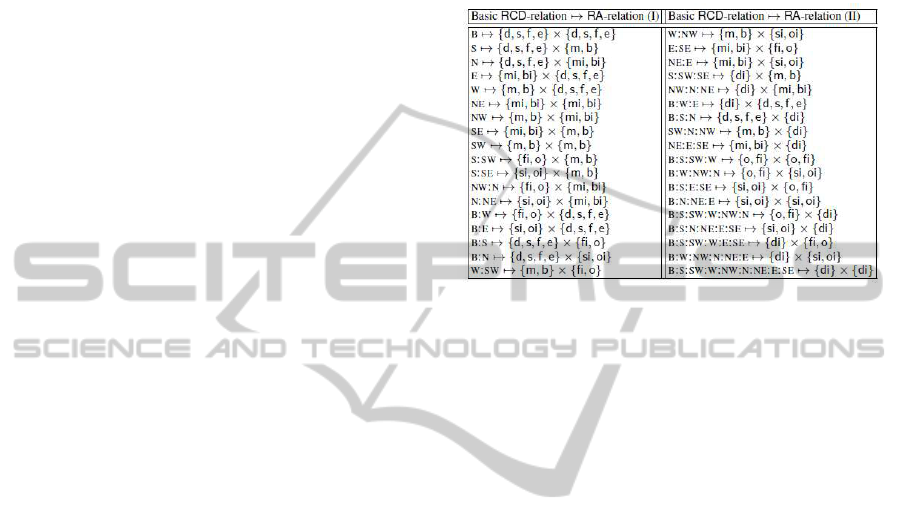
Figure 4: Translation from basic RCD-relations to RA-
relations via toRA mapping.
Figure 4 describes a translation function, called
toRA, to map a basic RCD-relation into the strongest
entailed RA-relation. This mapping can be extended
to translate arbitrary relations, constraints, and net-
works of RCD-calculus to their counterparts in RA,
preserving consistency. More precisely, given a dis-
junctive relation R, toRA(R) is obtained as the union
of the translation of the basic relations in R, while,
given an RCD-network N = (V,C), the corresponding
RA-network toRA(N) is obtained by replacing each
relation R
ij
in C by toRA(R
ij
). As the following the-
orem states, to decide the consistency of an RCD-
network N, one can compute the corresponding RA-
network toRA(N) and then apply any algorithm for
deciding the consistency of RA-networks (Navarrete
et al., 2011).
Theorem 1. An RCD-network N is consistent if and
only if the RA-network toRA(N) is consistent.
3.2 The Convex Fragment of RCD
In (Navarrete and Sciavicco, 2006), the authors prove
that the consistency problem for the RCD-calculus is
NP-complete, and they identify a tractable subset of
RCD-relations. A larger tractable fragment of RCD-
calculus, called convex RCD-calculus, has been iden-
tified in (Navarrete et al., 2011). Such a fragment
consists of all and only the RCD-relations R whose
translation toRA(R) is a convex RA-relation (convex
RCD-relations). It is possible to show that there exist
400 such relations.
As we already pointed out, the convex subclasses
ICAART 2012 - International Conference on Agents and Artificial Intelligence
158

Algorithm 3.1: the algorithm con-cRCD.
Require: a convex RCD-network N
1: N
r
← toRA(N);
2: N
x
← π
x
(N
r
); N
y
← π
y
(N
r
);
3: N
P
x
← toPA(N
x
); N
P
y
← toPA(N
y
);
4: If CSPAN(N
P
x
) or CSPAN(N
P
y
) returns an empty
network, then return ‘inconsistent’; otherwise, re-
turn ‘consistent’.
of IA, PA, and RA are tractable and PC-algorithms
can be used to decide their consistency. In particu-
lar, the following result holds for RA (Balbiani et al.,
1998):
Theorem 2. Let N be a convex RA-network. N is
path-consistent (resp., consistent) iff its projections
π
x
(N) and π
y
(N) are path-consistent (resp., consis-
tent). Moreover, if N is path consistent, then it is con-
sistent.
Making use of the above results, polynomial-time
algorithms to solve the consistency and the minimal-
ity problems for convex RCD-networks have been
proposed in (Navarrete et al., 2011). In the follow-
ing, we will exploit one of these algorithms, called
con-cRCD, that solves the two PA-networks corre-
sponding to a convex RCD-network. Such an algo-
rithm can be summarized as follows. Let N be a con-
vex RCD-network. First, it applies the mapping toRA
to get the convex RA-network N
r
corresponding to N.
Then, it computes the projections N
x
and N
y
of N
r
.
Next, it applies the mapping toPA to translate the con-
vex IA-networks N
x
and N
y
into two equivalent PA-
networks N
P
x
and N
P
y
with convex relations between
intervals endpoints. Such a mapping is based on the
list of the convex IA-relations and of their transla-
tions to PA given in (van Beek and Cohen, 1990).
Finally, the algorithm CSPAN (van Beek, 1992) is
applied to decide the consistency of the two convex
PA-networks in O(n
2
) (we assume that this algorithm
returns an empty network in case the input network
is inconsistent). It can be easily shown that such an
algorithm runs in O(n
2
). Algorithm 3.1 provides a
pseudocode encoding of con-cRCD.
4 CONVEX-METRIC RCD
In this section, we propose a tractable metric ex-
tension of the convex RCD-calculus, called convex-
metric RCD, to represent and to reason with both
qualitative cardinal constraints between rectangles
and metric constraints on the distance between the
endpoints of their projections.
4.1 STP
The main tool we use to deal with metric information
in convex-metric RCD is the STP formalism, which
was introduced in (Dechter et al., 1991) to process
metric information about time points. More precisely,
we use STP to elaborate information on the endpoints
of MBR projections onto the Cartesian axes.
Formally, an STP is specified by a constraint net-
work S = (P, M), where P is a set of point variables,
whose values range over a dense domain (we as-
sume it to be Q), and M is a set of binary metric
constraints over P. A metric constraint M
ij
= [q, q
′
]
(open and semi-open intervals can be used), with
q, q
′
∈ Q, on the distance between (the values of)
p
i
, p
j
∈ P states that p
j
− p
i
∈ [q, q
′
], or, equivalently,
that q ≤ p
j
− p
i
≤ q
′
. Hence, the constraint M
ij
de-
fines the set of possible values for the distance p
j
− p
i
.
In the constraint graph associated to S, M
ij
= [q, q
′
]
is represented by an edge from p
i
to p
j
labeled by
the rational interval [q, q
′
]. Unary metric constraints
restricting the domain of a point variable p
i
can be
encoded as binary constraints between p
i
and a spe-
cial starting-point variable with a fixed value, e.g., 0.
The universal constraint is ] − ∞, +∞[. The opera-
tions of composition (◦) and inverse (
−1
) of metric
constraints are computed by means of interval arith-
metic, that is, [q
1
, q
2
]◦ [q
3
, q
4
] = [q
1
+ q
3
, q
2
+ q
4
] and
[q
1
, q
2
]
−1
= [−q
2
, −q
1
]. Intersection of constraints
(intervals) is defined as usual.
Assuming such an interpretation of the operations
of composition, inverse, and intersection, Dechter et
al. (1991) showed that any PC-algorithm can be ex-
ploited to compute the minimal STP equivalent to
a given one, if any (if an inconsistency is detected,
the algorithm returns an empty network). In the fol-
lowing, we will denote such an algorithm by PC
stp
.
Making use of such a result, Meiri (1996) proposed
a formalism to combine qualitative constraints be-
tween points and intervals with (possibly disjunc-
tive) metric constraints between points (as in TCSP).
An easy special case arises when only convex PA-
constraints and STP-constraints are considered. Con-
vex PA-constraints can be encoded as STP-constraints
by means of the toSTP translation function described
in Table 1. The following result can be found in
Meiri (1996):
Theorem 3. Let N be a network with convex PA-
constraints and STP-constraints. If N is path-
consistent, then N is also consistent and its metric
constraints are minimal.
PC
stp
can thus be used to decide the consistency
of a network N satisfying the conditions of the above
A TRACTABLE FORMALISM FOR COMBINING RECTANGULAR CARDINAL RELATIONS WITH METRIC
CONSTRAINTS
159

theorem. To this end, it suffices to encode PA-
constraints into equivalent STP-constrains.
Table 1: Translation of convex PA-constraints to STP-
constraints via the toSTP mapping.
Convex PA relation STP constraint
p
i
< p
j
p
j
− p
i
∈ ]0, +∞[
p
i
≤ p
j
p
j
− p
i
∈ [0, +∞[
p
i
= p
j
p
j
− p
i
∈ [0, 0]
p
i
> p
j
p
j
− p
i
∈ ]−∞, 0[
p
i
≥ p
j
p
j
− p
i
∈ ]−∞, 0]
p
i
? p
j
p
j
− p
i
∈ ]−∞, +∞[
4.2 Integrating Convex RCD with STP
Combining RCD with STP makes it possible to ex-
press both directional constraints and metric con-
straints in a uniform framework. As an example, the
resulting formalism allows one to constrain the posi-
tion of a rectangle in the plane and to impose mini-
mum and/or maximum values to the width/height of
a given rectangle, or on the vertical/horizontal dis-
tances between the sides of two rectangles. Obvi-
ously, RCD-constraints and STP-constraints are not
totally independent, that is, RCD-constraints entail
some metric constraints and vice versa.
Example 3. Let a and b be two rectangle. We can
use the metric constraint 0 < a
+
x
− a
−
x
≤ 7 to state
that the maximum width of a is 7 and, similarly, we
can exploit the metric constraint 2 ≤ a
+
y
− a
−
y
to state
that the minimum height of a is 2 (leaving the max-
imum height unbounded). We can also express dis-
tance constraints between the boundaries of a and b.
We can constrain the horizontal distance between the
right side of a and the left side of b to be at least 3
by means of the constraint 3 ≤ b
−
x
− a
+
x
, and the ver-
tical distance between the upper side of a and the
bottom side of b to be greater than or equal to 0
by means of the constraint 0 ≤ b
−
y
− a
+
y
. The two
constraints together entail the basic RCD constraint
a{SW}b. Finally, some metric constraints can be
entailed by RCD ones. For instance, the convex re-
lation a{NW, N, NE, NW:N, NW:N:NE, N:NE}b im-
plies that 0 ≤ a
−
y
− b
+
y
.
If we allow one to combine arbitrary RCD-
constraints with metric constrains, then checking the
consistency of the resulting set of constraints turns out
to be an NP-complete problem (the consistency prob-
lem for RCD-networks is already NP-complete). To
preserve tractability, we restrict our attention to the
combination of convex RCD-constraints with STP-
constraints to establish the convex-metric RCD for-
malism.
Given a convex RCD-network N
c
= (V,C), we de-
note the sets of interval variables belonging to the pro-
jections π
x
(toRA(N
c
)) and π
y
(toRA(N
c
)) by V
x
and
V
y
, respectively. Moreover, we denote by P(V
x
) and
P(V
y
) the sets of point variables representing the end-
points of the interval variables in V
x
and V
y
, respec-
tively. A convex-metric RCD-network is formally de-
fined as follows.
Definition 2. A convex-metric RCD-network
(cmRCD-network) is an integrated qualitative and
metric constraint network N consisting of three
sub-networks (N
c
, S
x
, S
y
), where N
c
= (V,C) is a
convex RCD-network, and S
x
=
P(V
x
), M
x
and
S
y
=
P(V
y
), M
y
are two STPs.
The convex-metric RCD formalism we propose sub-
sumes the STP formalism and the convex RCD-
calculus. Moreover, it also generalizes the convex
fragment of the RA, since convex RA-relations are
expressible as convexPA-relations and these relations
can be, in turn, encoded into an STP.
Now, we provide an algorithm to solve the consis-
tency problem for cmRCD that runs in O(n
3
)
2
. First,
we extend the translation mapping toSTP of Table 1
to encode a convex PA-network N
P
into an STP S
by replacing each relation R
ij
in the network N
P
by
toSTP(R
ij
). By exploiting such a function, we can
generalize the algorithm con-cRCD of Section 3.2
to deal with both RCD- and STP-constrains (Algo-
rithm con-cmRCD). First, con-cmRCD computes
the PA-networks N
P
x
and N
P
y
, and then, making use
of information about convex RCD-relations encoded
as PA-relations, it looks for possible inconsistencies
between these constraints and the STP-constrains on
the same variables given in S
x
and S
y
that can be de-
tected at this stage. To this end, it translates the PA-
network N
P
x
(resp., N
P
y
) into an STP-network by ap-
plying the function toSTP, and then it uses the func-
tion intersect to compute the “intersection” between
toSTP(N
P
x
) and S
x
(resp., toSTP(N
P
y
) and S
y
). This
function simply intersects the intervals / metric con-
strains associated with the same pairs of variables in
the two STPs. If an interval intersection produces an
empty interval, then intersect returns an empty net-
work, and we can conclude that N is inconsistent.
Otherwise, we apply the path-consistency algorithm
to the two STPs computed at lines 4 and 5 independ-
2
A similar combination of qualitative and quantitative
networks is given by preconvex-augmented rectangle net-
works by Condotta (2000), that subsume cmRCD-networks.
An O(n
5
) algorithm for checking the consistency of these
networks has been devised by Condotta (Condotta, 2000).
We exploit the trade-off between expressiveness and com-
plexity to obtain a more efficient consistency checking al-
gorithm.
ICAART 2012 - International Conference on Agents and Artificial Intelligence
160

Algorithm 4.1: The algorithm con-cmRCD.
Require: a cmRCD-network N = (N
c
, S
x
, S
y
)
1: N
r
← toRA(N
c
);
2: N
x
← π
x
(N
r
), N
y
← π
y
(N
r
);
3: N
P
x
← toPA(N
x
), N
P
y
← toPA(N
y
);
4: xSTP ← intersect(toSTP(N
P
x
), S
x
);
5: ySTP ← intersect(toSTP(N
P
y
), S
y
);
6: if xSTP or ySTP is empty, then return ‘inconsis-
tent’;
7: xSTP
min
← PC
stp
(xSTP);
8: ySTP
min
← PC
stp
(ySTP);
9: If xSTP
min
or ySTP
min
is empty, then return ‘in-
consistent’; otherwise, return ‘consistent’.
ently. The following theorem proves that
con-cmRCD is sound and complete.
Theorem 4. Given a cmRCD-network N = (N
c
, S
x
,
S
y
), the algorithm con-cmRCD returns ‘consistent’
if and only if N is consistent.
Proof. We basically follow the steps of the algo-
rithm. By Theorem 1, N
c
is consistent if and only
if N
r
is consistent, and, by Theorem 2, N
r
is con-
sistent if and only if N
x
and N
y
are consistent (they
can be checked independently). Next, N
x
and N
y
are consistent if and only if N
P
x
and N
P
y
are consis-
tent, since there is no loss in information in the trans-
lations (van Beek and Cohen, 1990). The consis-
tency of N
P
x
and N
P
y
could be checked by comput-
ing the corresponding STPs and by applying PC
stp
.
However, we cannot apply PC
stp
directly to the STPs
toSTP(N
P
x
) and toSTP(N
P
x
) since the metric con-
straints of S
x
and S
y
must be taken into account.
Hence, we compute intersect(toSTP(N
P
x
), S
x
) and
intersect(toSTP(N
P
x
), S
y
). If one of them returns an
empty network, then N is inconsistent. Otherwise, we
independently apply PC
stp
to xSTP and ySTP. By
Theorem 3, if one of the two applications of PC
stp
re-
turns an empty network, then N is inconsistent; other-
wise, the path-consistent STPs xSTP
min
and ySTP
min
are consistent (and minimal), and thus N is consis-
tent.
Theorem 5. The complexity of the algorithm
con-cmRCD is O(Rn
3
), where n is the number of
variables and R is the maximum range of the network.
Proof. The translation via toRA, the generation of a
projection of a network, the transformation of a IA-
network into a RA-network via toPA and the last two
encodings via toSTP require O(n
2
) steps, since there
are O(n
2
) constraints and each constraint can be trans-
lated in constant time. The function toPA introduces
two variables for each interval variable, so xSTP and
ySTP have O(n) variables each. Finally, PC
stp
runs
in O(Rn
3
) time, so the overall complexity is O(Rn
3
)
time, where R is the maximum range of the network
(for more details about the complexity of achieving
path-consistency for combined networks see (Meiri,
1996)).
Once we have computed the path-consistent STPs
xSTP
min
and ySTP
min
with algorithm con-cmRCD,
we can build a solution to the convex-metric RCD-
network N by computing a solution for the points
in xSTP and ySTP, since the assignment for point
variables defines a consistent assignment for rectan-
gle variables (see Example 1). To this end, the al-
gorithm STP-SOLUTION by Gerevini and Cristani
(1997) (Gerevini and Cristani, 1997) can be used.
To illustrate the expressive power of the convex-
metric RCD-calculus and its potential applications,
we show an example regarding the design of 2D-
layouts.
Example 4. Uncle Scrooge wants to buy a plot of
land (p) to build a new money bin (m), an office (o), a
house (h) and a swimming pool (s) for Huey, Dewey,
and Louie. The surfaces of the buildings are supposed
to be rectangular, with sides aligned to the sides of
the plot, which also has a rectangular shape. Dur-
ing the feasibility study of the project, the following
requirements arose: i) the vertical and horizontal dis-
tance between the boundaries of p and any building
it contains must be at least 100m for reasons of pri-
vacy; ii) the surface area of m is 70m×70m; iii) m
must lie somewhere between the northwest zone and
the northeast zone of h, and the same w.r.t. o; iv) the
vertical distance between m and h (resp., o) must be
at least 100m because Uncle Scrooge does not want
to be disturbed too much by his employees; v) the sur-
face area of h is 100m×50m, while the surface area
of o is 30m×70m; vi) o must lie between the northeast
zone and east zone of h; vii) the horizontal distance
between o and h must be at least 60m and at most
80m so that Huey, Dewey, and Louie can play without
disturbing their uncle’s workers; viii) s is an olympic-
size swimming pool so its surface area has to be at
least 50m×25m and at most 100m×50m; ix) s must
be situated between the southwest zone and southeast
zone of h, and the same w.r.t. o; x) the vertical dis-
tance between s and h and between s and o must be at
least 50m.
Let us see howto represent the requirements of the
above example with a cmRCD-network. The qualita-
tive part of the network contains the following convex
RCD-contraints between variables p, m, h, o, and s
representing the plot and the buildings:
A TRACTABLE FORMALISM FOR COMBINING RECTANGULAR CARDINAL RELATIONS WITH METRIC
CONSTRAINTS
161

p
−
x
p
+
x
o
−
x
o
+
x
h
+
x
h
−
x
m
−
x
m
+
x
s
+
x
s
−
x
]-∞, 100]
]-∞, 100]
]-∞, 100]
[100, +∞[
[100, +∞[
[100, +∞[
[100, +∞[
]-∞, 0[
]-∞, 0[
]-∞, 0[
]-∞, 0[
]0, +∞[
]0, +∞[
]0, +∞[
[100, 100]
[30, 30]
[70, 70]
[50, 100]
]-∞, 0[
]-∞, 0[
]-∞, 0[
[60, 80]
]-∞, 100]
]0, +∞[
]0, +∞[
o
−
y
o
+
y
h
+
y
h
−
y
m
−
y
m
+
y
s
+
y
s
−
y
[100, +∞[
[50, 50]
[70, 70]
[25, 50]
[50, +∞[
[50, +∞[
[100, +∞[
]-∞, 0[
]-∞, 0[
]-∞, 0[
]-∞, 0[
]-∞, 0[
]-∞, 0[
]-∞, 0]
]-∞, 0[
]0, +∞[
]0, +∞[
]0, +∞[
]0, +∞[
]0, +∞[
]0, +∞[
[70, 70]
Figure 5: Graph representation of part of xSTP and part of ySTP of Example 4. For clarity, constraints involving p in ySTP
are omitted, as well as the universal constraint.
Implicit: “buildings must be inside the plot”:
oB p, hB p, mB p, sB p;
iii) m{NW, N, NW:N, NW:N:NE, N:NE, NE}h,
m{NW, N, NW:N, NW:N:NE, N:NE,NE}o;
vi) o{NE, NE:E, E}h;
ix) s{SW, S, SW:S, SW:S:SE, S:SE, SE} h,
s{SW, S, SW:S, SW:S:SE, S:SE, SE} o;
The quantitative part of the network contains the fol-
lowing metric constraints forming two STPs:
i) for all buildings b:
b
−
x
− p
−
x
≥ 100, p
+
x
− b
+
x
≥ 100,
b
−
y
− p
−
y
≥ 100, p
+
y
− b
+
y
≥ 100
ii) m
+
x
− m
−
x
= 70, m
+
y
− m
−
y
= 70;
iv) m
−
y
− h
+
y
≥ 100, m
−
y
− o
+
y
≥ 100;
v) h
+
x
− h
−
x
= 100, h
+
y
− h
−
y
= 50,
o
+
x
− o
−
x
= 30, o
+
y
− o
−
y
= 70;
vii) 60 ≤ o
−
x
− h
+
x
≤ 80;
viii) 50 ≤ s
+
x
− s
−
x
≤ 100, 25 ≤ s
+
y
− s
−
y
≤ 50
x) h
−
y
− s
+
y
≥ 50, o
−
y
− s
+
y
≥ 50.
By applying our consistency algorithm we can verify
that it is possible to realize the building project of the
example (the corresponding cmRCD-network is con-
sistent). We can also determine the minimum area
that the plot should have by using the minimal net-
works xSTP
min
and ySTP
min
: in our example the min-
imum area of p is 390m×515m while the maximum
area is unbounded. The STPs xSTP and ySTP, com-
puted by steps 4 and 5 of our algorithm, are sketched
in Figure 5, while a solution of the problem is illus-
trated by Figure 6, showing the minimum feasible val-
ues for the point variables. To simplify, we suppose
that the origin of the reference system is the lower-left
vertex of the plot, since the plot encloses all the build-
m
o
s
h
335
415
245
175
125
100
y
225
180
250 260 290
100
200
x
165
p
0 390
515
70
70
70
30
100
50
50
25
Figure 6: A solution to the cmRCD-network corresponding
to Example 4.
ing and there is no constraint between the plot and the
space around it.
5 CONCLUSIONS
In this paper, we have proposed a quite expressive,
but tractable, metric extension of RCD (cmRCD),
that integrates STP-constraints with convex RCD-
constraints. cmRCD allows one to constrain the posi-
tion of a rectangle in the plane, its width/height, and
the vertical/horizontal distance between the sides of
two rectangles, as well as to represent cardinal rela-
tions between rectangles. We have devised an O(n
3
)
consistency-checking algorithm, and we have showed
how a spatial realization of a network can be built.
As for future work, we plan to extend cmRCD
with topological relations to improve its expressive-
ICAART 2012 - International Conference on Agents and Artificial Intelligence
162

ness (similar results can be found in (Gerevini and
Renz, 2002; Liu et al., 2009)). The problem of identi-
fying maximal tractable subsets of RCD is still open.
It would be interesting to search for tractable classes
(strictly) including the convex fragment.
ACKNOWLEDGEMENTS
This work has been partially supported by the Span-
ish Ministry of Science and Innovation, the European
Regional Development Fund of the European Com-
mission under grant TIN2009-14372-C03-01, and
the Spanish MEC through the project 15277/PI/10,
funded by Seneca Agency of Science and Technol-
ogy of the Region of Murcia within the II PCTRM
2007-2010. Finally, Guido Sciavicco and Angelo
Montanari were also partially founded by the Span-
ish fellowship ‘Ramon y Cajal’ RYC-2011-07821and
by the Italian PRIN project Innovative and multi-
disciplinary approaches for constraint and preference
reasoning, respectively.
REFERENCES
Allen, J. (1983). Maintaining knowledge about temporal
intervals. Communications of the ACM, 26(11):832–
843.
Balbiani, P., Condotta, J., and del Cerro, L. (1998). A model
for reasoning about bidimensional temporal relations.
In Proceedings of KR-98, pages 124–130.
Balbiani, P., Condotta, J., and del Cerro, L. (2002).
Tractability results in the block algebra. Journal of
Logic and Computation, 12(5):885–909.
Baykan, C. and Fox, M. (1997). Spatial synthesis by dis-
junctive constraint satisfaction. Artificial Intelligence
for Engineering Design, Analysis and Manufacturing,
11(4):245–262.
Broxvall, M. (2002). A method for metric temporal reason-
ing. In Proceedings of AAAI-02, pages 513–518.
Cohn, A. and Hazarika, S. (2001). Qualitative spatial rep-
resentation and reasoning: An overview. Fundamenta
Informaticae, 46(1-2):1–29.
Condotta, J. F. (2000). The augmented interval and rectan-
gle networks. In Proceedings of KR-00, pages 571–
579.
Dechter, R., Meiri, I., and Pearl, J. (1991). Temporal con-
straint networks. Artificial Intelligence, 49(1-3):61–
95.
El-Geresy, B. and Abdelmoty, A. (2001). Qualitative rep-
resentations in large spatial databases. Proceedings of
IDEAS-01, pages 68–75.
Frank, A. (1996). Qualitative spatial reasoning: Cardinal
directions as an example. International Journal of Ge-
ographical Information Science, 10(3):269–290.
Gatterbauer, W. and Bohunsky, P. (2006). Table extraction
using spatial reasoning on the CSS2 visual box model.
In Proceedings of AAAI-06, volume 2.
Gerevini, A. and Cristani, M. (1997) On finding a solution
in temporal constraint satisfaction problems. In Pro-
ceedings of IJCAI-97, pages 1460–1465.
Gerevini, A. and Renz, J. (2002). Combining topological
and size information for spatial reasoning. Artificial
Intelligence, 137(1-2):1–42.
Goyal, R. (2000). Similarity assessment for cardinal di-
rections between extended spatial objects. PhD the-
sis, University of Maine, Dept. of Spatial Information
Science and Engineering.
Goyal, R. and Egenhofer, M. (2000). Consistent queries
over cardinal directions across different levels of de-
tail. In Proceedings of DEXA-00, pages 876–880.
Liu, W., Li, S., and Renz, J. (2009). Combining RCC-8 with
qualitative direction calculi: Algorithms and complex-
ity. In Proceedings of IJCAI-09, pages 854–859.
Liu, W., Zhang, X., Li, S., and Ying, M. (2010). Reasoning
about cardinal directions between extended objects.
Artificial Intelligence, 174:951–983.
Mackworth, A. (1977). Consistency in networks of rela-
tions. Artificial Intelligence, 8(1):99–118.
Meiri, I. (1996). Combining qualitative and quantitative
constraints in temporal reasoning. Artificial Intelli-
gence, 87(1-2):343–385.
Navarrete, I., Morales, A., Sciavicco, G., and Cardenas-
Viedma, M. (2011). Spatial reasoning with rect-
angular cardinal relations. Technical Report TR-
DIIC 2/11, Departamento de Ingenieria de la Informa-
cion y las Comunicaciones. Universidad de Murcia.
http://sites.google.com/site/aikespatial/RCDC.
Navarrete, I. and Sciavicco, G. (2006). Spatial reason-
ing with rectangular cardinal direction relations. In
Proceedings of the ECAI-06 Workshop on Spatial and
Temporal Reasoning, pages 1–10.
Papadias, D. and Theodoridis, Y. (1997). Spatial relations,
minimum bounding rectangles, and spatial data struc-
tures. International Journal of Geographical Informa-
tion Science, 11(2):111–138.
Skiadopoulos, S., Giannoukos, C., Sarkas, N., Vassiliadis,
P., Sellis, T., and Koubarakis, M. (2005). Comput-
ing and managing cardinal direction relations. IEEE
Transactions on Knowledge and Data Engineering,
17(12):1610–1623.
Skiadopoulos, S. and Koubarakis, M. (2005). On the con-
sistency of cardinal directions constraints. Artificial
Intelligence, 163(1):91–135.
van Beek, P. (1992). Reasoning about qualitative temporal
information. Artificial Intelligence, 58(1-3):297–326.
van Beek, P. and Cohen, R. (1990). Exact and approximate
reasoning about temporal relations. Computation In-
telligence, 6(3):132–147.
Vilain, M. and Kautz, H. (1986). Constraint propagation
algorithms for temporal reasoning. In Proceedings of
AAAI-86, pages 377–382.
A TRACTABLE FORMALISM FOR COMBINING RECTANGULAR CARDINAL RELATIONS WITH METRIC
CONSTRAINTS
163
