
ON UNSUPERVISED NEAREST-NEIGHBOR REGRESSION
AND ROBUST LOSS FUNCTIONS
Oliver Kramer
Department for Computer Science, Carl von Ossietzky Universit
¨
at Oldenburg,
Uhlhornsweg 84, 26129 Oldenburg, Germany
Keywords:
Non-linear dimensionality reduction, Manifold learning, Unsupervised regression, K-nearest neighbor
regression.
Abstract:
In many scientific disciplines structures in high-dimensional data have to be detected, e.g., in stellar spectra,
in genome data, or in face recognition tasks. We present an approach to non-linear dimensionality reduction
based on fitting nearest neighbor regression to the unsupervised regression framework for learning of low-
dimensional manifolds. The problem of optimizing latent neighborhoods is difficult to solve, but the UNN
formulation allows an efficient strategy of iteratively embedding latent points to fixed neighborhood topolo-
gies. The choice of an appropriate loss function is relevant, in particular for noisy, and high-dimensional data
spaces. We extend unsupervised nearest neighbor (UNN) regression by the ε-insensitive loss, which allows to
ignore residuals under a threshold defined by ε. In the experimental part of this paper we test the influence of
ε on the final data space reconstruction error, and present a visualization of UNN embeddings on test data sets.
1 INTRODUCTION
Dimensionality reduction and manifold learning have
an important part to play in the understanding of data.
In this work we extend the two constructive heuris-
tics for dimensionality reduction called unsupervised
K-nearest neighbor regression (Kramer, 2011) by ro-
bust loss functions. Meinicke proposed a general
unsupervised regression framework for learning low-
dimensional manifolds (Meinicke, 2000). The idea
is to reverse the regression formulation such that low-
dimensional data samples in latent space optimally re-
construct high-dimensional output data. We take this
framework as basis for an iterative approach that fits
KNN to this unsupervised setting in a combinatorial
variant. The manifold problem we consider is a map-
ping F : y → x corresponding to the dimensionality re-
duction for data points y ∈ Y ⊂ R
d
, and latent points
x ∈ X ⊂ R
q
with d > q. The problem is a hard op-
timization problem as the latent variables X are un-
known.
In Section 2 we will review related work in di-
mensionality reduction, unsupervised regression, and
KNN regression. Section 3 presents the concept of
UNN regression, and two iterative strategies that are
based on fixed latent space topologies. In Section 4
we extend UNN to robust loss functions, i.e., the ε-in-
sensitive loss. Conclusions are drawn in Section 5.
2 RELATED WORK
Dimensionality reduction is the problem of learn-
ing a mapping from high-dimensional data space to
a space with lower dimensions, while losing as lit-
tle information as possible. Many dimensionality
reduction methods have been proposed in the past,
a very famous one is principal component analysis
(PCA), which assumes linearity of the manifold (Jol-
liffe, 1986; Pearson, 1901). An extension for learning
non-linear manifolds is kernel PCA (Sch
¨
olkopf et al.,
1998) that projects the data into a Hilbert space. Fur-
ther famous approaches for dimensionality reduction
are Isomap by Tenenbaum et al. (Tenenbaum et al.,
2000), locally linear embedding (LLE) by Roweis and
Saul (Roweis and Saul, 2000), and principal curves by
Hastie and Stuetzle (Hastie and Stuetzle, 1989).
2.1 Unsupervised Regression
The work on unsupervised regression for dimen-
sionality reduction started with Meinicke (Meinicke,
2000), who introduced the corresponding algorith-
mic framework for the first time. In this line of
164
Kramer O..
ON UNSUPERVISED NEAREST-NEIGHBOR REGRESSION AND ROBUST LOSS FUNCTIONS.
DOI: 10.5220/0003749301640170
In Proceedings of the 4th International Conference on Agents and Artificial Intelligence (ICAART-2012), pages 164-170
ISBN: 978-989-8425-95-9
Copyright
c
2012 SCITEPRESS (Science and Technology Publications, Lda.)

research early work concentrated on non-parametric
kernel density regression, i.e., the counterpart of the
Nadaraya-Watson estimator (Meinicke et al., 2005)
denoted as unsupervised kernel regression (UKR).
Let Y = (y
1
,...y
N
) with y
i
∈ R
d
be the matrix of
high-dimensional patterns in data space. We seek for
a low-dimensional representation, i.e., a matrix of la-
tent points X = (x
1
,...x
N
), so that a regression func-
tion f applied to X point-wise optimally reconstructs
the patterns, i.e., we search for an X that minimizes
the reconstruction in data space. The optimization
problem can be formalized as follows:
minimize E(X) =
1
N
kY −f(x; X)k
2
. (1)
E(X) is called data space reconstruction error
(DSRE). Latent points X define the low-dimensional
representation. The regression function applied to the
latent points should optimally reconstruct the high-
dimensional patterns. The regression model f induces
its capacity, i.e., the kind of structure it is able to rep-
resent, to the mapping.
The unsupervised regression framework works as
follows:
• Initialize latent variables X = (x
1
,...x
N
),
• minimize E(X) w.r.t. DSRE employing an opti-
mization / cross-validation scheme,
• evaluate embedding.
Many regression methods can fit into this framework.
A typical example is unsupervised kernel regression,
analyzed by Klanke and Ritter (Klanke and Ritter,
2007), but further methods can also be employed.
Klanke and Ritter (Klanke and Ritter, 2007) intro-
duced an optimization scheme based on LLE, PCA,
and leave-one-out cross-validation (LOO-CV) for
UKR. Carreira-Perpi
˜
n
´
an and Lu (Carreira-Perpi
˜
n
´
an
and Lu, 2010) argue that training of non-parametric
unsupervised regression approaches is quite expen-
sive, i.e., O(N
3
) in time, and O(N
2
) in memory. Para-
metric methods can accelerate learning, e.g., unsuper-
vised regression based on radial basis function net-
works (RBFs) (Smola et al., 2001), Gaussian pro-
cesses (Lawrence, 2005), and neural networks (Tan
and Mavrovouniotis, 1995).
2.2 KNN Regression
In the following, we give a short introduction to K-
nearest neighbor regression that is basis of the UNN
approach. KNN is a technique with long tradition.
It was first mentioned by Fix and Hodges (Fix and
Hodges, 1951) in the fifties in an unpublished US
Air Force School of Aviation Medicine report as non-
parametric classification technique. Cover and Hart
(Cover and Hart, 1967) investigated the approach ex-
perimentally in the sixties. Interesting properties have
been found, e.g., that for K = 1, and N → ∞, KNN is
bound by the Bayes error rate.
The problem in regression is to predict output val-
ues y ∈ R
d
of given input values x ∈ R
q
based on sets
of N input-output examples ((x
1
,y
1
),...,(x
N
,y
N
)).
The goal is to learn a function f : x → y known as
regression function. We assume that a data set con-
sisting of observed pairs (x
i
,y
i
) ∈ X × Y is given. For
a novel pattern x
0
KNN regression computes the mean
of the function values of its K-nearest neighbors:
f
knn
(x
0
) =
1
K
∑
i∈N
K
(x
0
)
y
i
(2)
with set N
K
(x
0
) containing the indices of the K-
nearest neighbors of x
0
. The idea of KNN is based
on the assumption of locality in data space: In lo-
cal neighborhoods of x patterns are expected to have
similar output values y (or class labels) compared to
f(x). Consequently, for an unknown x
0
the label must
be similar to the labels of the closest patterns, which
is modeled by the average of the output value of the
K nearest samples. KNN has been proven well in
various applications, e.g., in the detection of quasars
based on spectroscopic data (Gieseke et al., 2010).
3 UNSUPERVISED KNN
REGRESSION
In this section we introduce the iterative strategy for
UNN regression (Kramer, 2011) that is based on
minimization of the data space reconstruction error
(DSRE).
3.1 Concept
An UNN regression manifold is defined by variables
x ∈ X ⊂ R
q
with unsupervised formulation of an
UNN regression manifold
f
UNN
(x;X) =
1
K
∑
i∈N
K
(x,X)
y
i
. (3)
Matrix X contains the latent points x that define the
manifold, i.e., the low-dimensional representation of
data Y. Parameter x is the location where the function
is evaluated. An optimal UNN regression manifold
minimizes the DSRE
minimize E(X) =
1
N
kY −f
UNN
(x;X)k
2
F
, (4)
ON UNSUPERVISED NEAREST-NEIGHBOR REGRESSION AND ROBUST LOSS FUNCTIONS
165
with Frobenius norm
kAk
2
F
=
v
u
u
t
d
∑
i=1
N
∑
j=1
|a
i j
|
2
. (5)
In other words: an optimal UNN manifold consists
of low-dimensional points X that minimize the recon-
struction of the data points Y w.r.t. the KNN regres-
sion method. Regularization in UNN regression is not
as important as regularization in other methods that fit
into the unsupervised regression framework. For ex-
ample, in UKR regularization means penalizing ex-
tension in latent space with E
p
(X) = E(X) + λkXk,
and weight λ (Klanke and Ritter, 2007). In KNN re-
gression moving the low-dimensional data samples
infinitely apart from each other does not have the
same effect as long as we can still determine the K-
nearest neighbors. But for practical purposes (limi-
tation of size of numbers) it might be reasonable to
restrict continuous KNN latent spaces as well, e.g., to
x ∈ [0,1]
q
. In the following section fixed latent space
topologies are used that do not require further regu-
larization.
3.2 Iterative Strategy 1
For KNN not the absolute positions of data samples
in latent space are relevant, but the relative positions
that define the neighborhood relations. This perspec-
tive reduces the problem to a combinatorial search for
neighborhoods N
K
(x
i
,X) with i = 1, . . . , N that can
be solved by testing all combinations of K-element
subsets of N elements.The problem is still difficult to
solve, in particular for high dimensions.
The idea of our first iterative strategy (UNN 1) is
to iteratively assign the data samples to a position in
an existing latent space topology that leads to the low-
est DSRE. We assume fixed neighborhood topologies
with equidistant positions in latent space, and there-
fore restrict the optimization problem of Equation (3)
to a search in a subset of latent space.
As a simple variant we consider the linear case of
the latent variables arranged equidistantly on a line
x ∈ R . In this simplified case only the order of the el-
ements is important. The first iterative strategy works
as follows:
1. Choose one element y ∈ Y,
2. test all
ˆ
N + 1 intermediate positions of the
ˆ
N em-
bedded elements
ˆ
Y in latent space,
3. choose the latent position that minimizes E(X),
and embed y,
4. remove y from Y, add y to
ˆ
Y, and repeat from
Step 1 until all elements have been embedded.
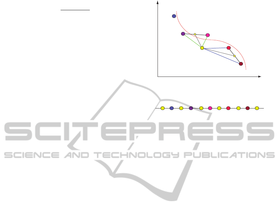
x
y
y
1
2
latent space
data space
x x x x x
1 2 3 4 5 6
f(x )
3
f(x )
5
y
Figure 1: UNN 1: illustration of embedding of a low-
dimensional point to a fixed latent space topology w.r.t. the
DSRE testing all
ˆ
N +1 positions.
Figure 1 illustrates the
ˆ
N + 1 possible embeddings of
a data sample into an existing order of points in latent
space (yellow/bright circles). The position of element
x
3
results in a lower DSRE with K = 2 than the po-
sition of x
5
, as the mean of the two nearest neighbors
of x
3
is closer to y than the mean of the two nearest
neighbors of x
5
.
Each DSRE evaluation takes Kd computations. It
is easily possible to save the K nearest neighbors in
latent space in a list, so that the search for indices
N
K
(x,X) takes O(1) time. The embedding of N el-
ements takes (N + 2) · ((N + 1)/2) · Kd steps, i.e.,
O(N
2
) time.
3.3 Iterative Strategy 2
The iterative approach introduced in the last section
tests all intermediate positions of previously embed-
ded latent points. We proposed a second iterative vari-
ant (UNN 2) that only tests the neighbored intermedi-
ate positions in latent space of the nearest embedded
point y
∗
∈
ˆ
Y in data space (Kramer, 2011). The sec-
ond iterative strategy works as follows:
1. Choose one element y ∈ Y,
2. look for the nearest y
∗
∈
ˆ
Y that has already been
embedded (w.r.t. distance measure like Euclidean
distance),
3. choose the latent position next to x
∗
that mini-
mizes E(X) and embed y,
4. remove y from Y, add y to
ˆ
Y, and repeat from
Step 1 until all elements have been embedded.
ICAART 2012 - International Conference on Agents and Artificial Intelligence
166
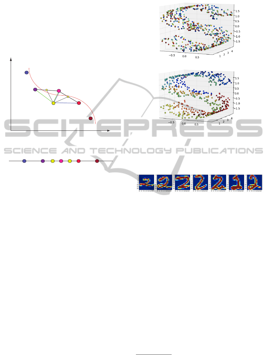
Figure 2 illustrates the embedding of a 2-
dimensional point y (yellow) left or right of the near-
est point y
∗
in data space. The position with the low-
est DSRE is chosen. In comparison to UNN 1,
ˆ
N dis-
tance comparisons in data space have to be computed,
but only two positions have to be tested w.r.t. the
data space reconstruction error. UNN 2 computes the
y
y
1
2
latent space
data space
x x
3 4
f(x )
3
f(x )
4
y
y
*
x
*
Figure 2: UNN 2: testing only the neighbored positions of
the nearest point y
∗
in data space.
nearest embedded point y
∗
for each data point taking
(N + 1) · (N/2) · d steps. Only for the two neighbors
the DSRE has to be computed, resulting in an overall
number of (N + 1) · N/2 · d + N · 2Kd steps. Hence,
UNN 2 takes O(N
2
) time for the whole embedding.
3.4 Experiments
In the following, we present a short experimental
evaluation of UNN regression on a 3-dimensional S
data set (3D-S), and a test problem from the USPS
digits data set (Hull, 1994). The 3D-S variant without
a hole consists of 500 data points. Figure 3(a) shows
the order of elements of the 3D-S data set at the begin-
ning. The corresponding embedding with UNN 1 and
K = 10 is shown in Figure 3(b). Similar colors corre-
spond to neighbored points in latent space. Figure 4
shows the embedding of 100 data samples of 256-
dimensional (16 x 16 pixels) images of handwritten
digits (2’s). We embed a one-dimensional manifold,
and show the high-dimensional data that is assigned
to every 14th latent point. We can observe that neigh-
bored digits are similar to each other, while digits that
are dissimilar are further away from each other in la-
tent space.
(a)
(b)
Figure 3: Results of UNN on 3D-S: (a) the unsorted S at the
beginning, (b) the embedded S with UNN 1 and K = 10.
Similar colors represent neighborhood relations in latent
space.
Figure 4: UNN 2 embeddings of 100 digits (2’s) from the
USPS data set. The images are shown that are assigned to
every 14th embedded latent point. Similar digits are neigh-
bored in latent space.
4 ROBUST LOSS FUNCTIONS
Loss functions have an important part to play in ma-
chine learning, as they define the error and thus the
design objective. In this section we introduce the ε-
insensitive loss for UNN regression.
4.1 ε-Insensitive Loss
In case of noisy data sets over-fitting effects may oc-
cur. The employment of the ε-insensitive loss al-
lows to ignore errors beyond a level of ε, and avoids
over-fitting to curvatures of the data that may only be
caused by noise effects
1
. With the design of a loss
function, the emphasis of outliers can be controlled.
First, the residuals are computed. In case of unsuper-
1
Of course, it is difficult to decide, and subject to the
application domain, if the curvature of the data manifold is
substantial or noise.
ON UNSUPERVISED NEAREST-NEIGHBOR REGRESSION AND ROBUST LOSS FUNCTIONS
167

vised regression, the error is computed in two steps:
1. The distance function δ : R
q
×R
d
→ R maps the
difference between the prediction f (x) and the de-
sired output value y to a value according to the
distance w.r.t. a certain measure. We employ the
Minkowski metric:
δ(x,y) =
N
∑
i=1
|f(x
i
) −y
i
)|
!
1/p
, (6)
which corresponds to the Manhattan distance for
p = 1, and to the Euclidean distance for p = 2.
2. The loss function L : R → R maps the residu-
als to the learning error. With the design of the
loss function the influence of residuals can be con-
trolled. In the best case the loss function is chosen
according to the needs of the underlying data min-
ing model. Often, low residuals are penalized less
than high residuals (e.g. with a quadratic func-
tion). We will concentrate on the ε-insensitive loss
in the following.
Let r be the residual, i.e., the distance δ in data space.
L
1
and L
2
loss functions are often employed, see the
Frobenius norm (Equation 5). The L
1
loss is defined
as
L
1
(r) = krk, (7)
and L
2
is defined as
L
2
(r) = r
2
. (8)
We will use the L
2
loss for measuring the final DSRE,
but concentrate on the ε-insensitive loss L
ε
during
training of the UNN model. The L
ε
is defined as:
L
ε
(r) =
0 if |r| < ε
|r| − ε if |r| ≥ ε
(9)
L
ε
is not differentiable at |r| = ε.
4.2 Experiments
In the following, we concentrate on the influence of
loss functions on the UNN embedding. For this sake,
we employ two kinds of ways to evaluate the final em-
bedding: We measure the final L
2
-based DSRE, visu-
alize the results by colored embeddings, and show the
latent order of the embedded objects. We concentrate
on two data sets, i.e., a 3D-S data set with noise, and
the USPS handwritten digits.
4.2.1 3D-S with Noise
In the first experiment, we concentrate on the 3D-S
data set. Noise is modeled by multiplying each data
point of the 3D-S with a random value drawn from
the Gaussian distribution: y
0
= N (0,σ) · y. Table 1
shows the experimental results of UNN 1 and UNN 2
concentrating on the ε-insensitive loss for K = 5, and
Minkowski metric with p = 2 on the 3D-S data set
with hole (3D-S
h
). The left part shows the results
for 3D-S without noise, the right part shows the re-
sults with noise (σ = 5.0). At first, we concentrate on
the experiments without noise. We can observe that
(1) the DSRE achieved by UNN 1 is minimal for the
lowest ε, and (2), for UNN 2 low DSRE values are
achieved with increasing ε (to a limit as of ε = 3.0),
but the best DSRE of UNN 2 is worse than the best of
UNN 1. Observation (1) can be explained as follows.
Without noise for UNN 1 ignoring residuals is disad-
vantageous: all intermediate positions are tested, and
a good local optimum can be reached. For observation
(2) we can conclude that a way against local optima
of UNN 2 is to ignore residuals.
For the experiments with noise of the magnitude
σ = 5.0 we can observe a local DSRE minimum: for
ε = 0.8 in case of UNN 1, and ε = 3.0 in case of
UNN 2. For UNN 1 local optima caused by noise can
be avoided by ignoring residuals, for UNN 2 this is al-
ready the case without noise. Furthermore, for UNN 2
we observe the optimum at the same level of ε.
Table 1: Influence of the ε-insensitive loss on final DSRE
(L
2
) of UNN for problem 3D-S
h
with, and without noise
σ = 0.0 σ = 5.0
ε
UNN 1 UNN 2 UNN 1 UNN 2
0.2 47.432 77.440 79.137 85.609
0.4 48.192 77.440 79.302 85.609
0.6 51.807 76.338 78.719 85.609
0.8 50.958 76.338 77.238 84.422
1.0 64.074 76.427 79.486 84.258
2.0 96.026 68.371 119.642 82.054
3.0 138.491 50.642 163.752 80.511
4.0 139.168 50.642 168.898 82.144
5.0 139.168 50.642 169.024 83.209
10.0 139.168 50.642 169.024 83.209
Figures 5 (a) and (b) show embeddings of UNN 1
and UNN 2 without noise, and the settings ε = 0.2,
and ε = 3.0, corresponding to the settings of Table 1
that are shown in bold. Similar colors correspond to
neighbored embeddings in latent space. The visual-
ization shows that for both embeddings neighbored
points in data space have similar colors, i.e., they cor-
respond to neighbored latent points. The UNN 1 em-
bedding results in a lower DSRE. This can hardly
be recognized from the visualization. Only the blue
points of UNN 2 seem to be distributed on the upper
and lower part of the 3D-S, which may represent a
local optimum.
Figures 6 (a) and (b) show the visualization of the
ICAART 2012 - International Conference on Agents and Artificial Intelligence
168
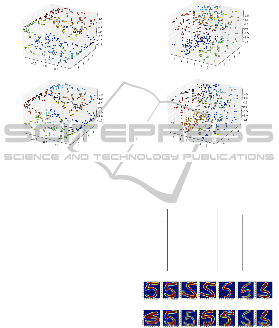
(a)
(b)
Figure 5: Visualization of the best UNN 1 and UNN 2 em-
beddings (lowest DSRE, bold values in Table 1) of 3D-S
h
without noise.
UNN embeddings on the noisy 3D-S. The structure
of the 3-dimensional S is obviously disturbed. Never-
theless, neighbored parts in data space are assigned to
similar colors. Again, the UNN 1 embedding seems
to be slightly better than the UNN 2 embedding, blue
points can again be observed at different parts of the
structure, representing local optima.
4.2.2 USPS Digits
To demonstrate the effect of the ε-insensitive loss for
data spaces with higher dimensions, we employ the
USPS handwritten digits data set with d = 256 again
by showing the DSRE, and presenting a visualization
of the embeddings. Table 2 shows the final DSRE
(w.r.t. the L
2
-loss) after training with the ε-insensitive
loss with various parameterizations for ε. We used the
setting K = 10, and p = 10.0 for the Minkowski met-
ric. The results for digit 5 show that a minimal DSRE
has been achieved for ε = 3.0 in case of UNN 1, and
ε = 5.0 for UNN 2 (a minimum of R = 429.75561
was found for ε = 4.7). Obviously, both methods
can profit from the use of the ε-insensitive loss. For
digit 7, and UNN 1 ignoring small residuals does not
seem to improve the learning result, while for UNN 2
ε = 4.0 achieves the best embedding.
Figure 7 shows two UNN 2 embeddings of the
handwritten digits data set for ε = 2.0, and ε = 20.0.
(a)
(b)
Figure 6: Visualization of the best UNN 1 and UNN 2
embeddings (lowest DSRE, bold values in Table 1) of 3D-
S
h
with noise σ = 5.0.
Table 2: Influence of ε-insensitive loss on final DSRE of
UNN on the digits data set.
digits 5’s digits 7’s
ε
UNN 1 UNN 2 UNN 1 UNN 2
0.0 423.8 440.2 225.4 222.8
1.0 423.8 440.2 225.4 222.8
2.0 423.8 440.2 225.6 222.8
3.0 423.5 440.2 238.1 221.0
4.0 441.3 440.2 262.1 218.2
5.0 488.7 432.3 264.8 221.4
6.0 496.9 434.2 265.6 220.8
10.0 494.6 434.3 268.4 220.8
(a)
(b)
Figure 7: Comparison of UNN 2 embeddings of 5’s from
the handwritten digits data set. The figures show every 14th
embedding of the sorting w.r.t. 100 digits for ε = 2.0, and
ε = 20.0.
For both settings similar digits are neighbored in la-
tent space. But we can observe that for ε = 20.0 a
ON UNSUPERVISED NEAREST-NEIGHBOR REGRESSION AND ROBUST LOSS FUNCTIONS
169

broader variety in the data set is covered. The loss
function does not concentrate on fitting to noisy parts
of the data, but has the capacity to concentrate on the
important structures of the data.
5 CONCLUSIONS
Fast dimensionality reduction methods are required
that are able to process huge data sets, and large
dimensions. With UNN regression we have fitted
well-known established regression technique into the
unsupervised setting for dimensionality reduction.
The two iterative UNN strategies are efficient meth-
ods to embed high-dimensional data into fixed one-
dimensional latent space. We have introduced two
iterative local variants that turned out to be perfor-
mant on test problems in first experimental analy-
ses. UNN 1 achieves lower DSREs, but UNN 2 is
slightly faster because of the multiplicative constants
of UNN 1. We concentrated on the employment of the
ε-insensitive loss, and its influence on the DSRE. It
could be observed that both iterative UNN regression
strategies could benefit from the ε-insensitive loss, in
particular the iterative variant UNN 2 could be im-
proved employing a loss with ε > 0. Obviously, local
optima can be avoided. The experimental results have
shown that this effect cannot only be observed for
low-dimensional data with noise, but also for high-
dimensional, i.e., the digits data set.
Our future work will concentrate on the analysis
of local optima of UNN embeddings, and on possible
extensions to guarantee global optimal solutions. This
work will include the analysis of stochastic global
search variants. Furthermore, the UNN strategies
will be extended to latent topologies with higher di-
mensionality. Another possible extension of UNN is
a continuous backward mapping from latent to data
space f : x → y employing a distance-weighted vari-
ant of KNN. A backward mapping can be used for
generating high-dimensional data based on sampling
in latent space.
REFERENCES
Carreira-Perpi
˜
n
´
an, M.
´
A. and Lu, Z. (2010). Parametric di-
mensionality reduction by unsupervised regression. In
Conference on Computer Vision and Pattern Recogni-
tion (CVPR), pages 1895–1902.
Cover, T. and Hart, P. (1967). Nearest neighbor pattern clas-
sification. IEEE Transactions on Information Theory,
13:21– 27.
Fix, E. and Hodges, J. (1951). Discriminatory analysis, non-
parametric discrimination: Consistency properties. 4.
Gieseke, F., Polsterer, K. L., Thom, A., Zinn, P., Bomanns,
D., Dettmar, R.-J., Kramer, O., and Vahrenhold, J.
(2010). Detecting quasars in large-scale astronomi-
cal surveys. In International Conference on Machine
Learning and Applications (ICMLA), pages 352–357.
Hastie, Y. and Stuetzle, W. (1989). Principal curves.
Journal of the American Statistical Association,
85(406):502–516.
Hull, J. (1994). A database for handwritten text recognition
research. IEEE Trans. on PAMI, 5(16):550–554.
Jolliffe, I. (1986). Principal component analysis. Springer
series in statistics. Springer, New York.
Klanke, S. and Ritter, H. (2007). Variants of unsupervised
kernel regression: General cost functions. Neurocom-
puting, 70(7-9):1289–1303.
Kramer, O. (2011). Dimensionalty reduction by unsuper-
vised nearest neighbor regression. In Proceedings of
the 10th International Conference on Machine Learn-
ing and Applications (ICMLA). IEEE, to appear.
Lawrence, N. D. (2005). Probabilistic non-linear principal
component analysis with gaussian process latent vari-
able models. Journal of Machine Learning Research,
6:1783–1816.
Meinicke, P. (2000). Unsupervised Learning in a General-
ized Regression Framework. PhD thesis, University of
Bielefeld.
Meinicke, P., Klanke, S., Memisevic, R., and Ritter, H.
(2005). Principal surfaces from unsupervised kernel
regression. IEEE Trans. Pattern Anal. Mach. Intell.,
27(9):1379–1391.
Pearson, K. (1901). On lines and planes of closest fit to
systems of points in space. Philosophical Magazine,
2(6):559–572.
Roweis, S. T. and Saul, L. K. (2000). Nonlinear dimension-
ality reduction by locally linear embedding. Science,
290:2323–2326.
Sch
¨
olkopf, B., Smola, A., and M
¨
uller, K.-R. (1998). Non-
linear component analysis as a kernel eigenvalue prob-
lem. Neural Computation, 10(5):1299–1319.
Smola, A. J., Mika, S., Sch
¨
olkopf, B., and Williamson,
R. C. (2001). Regularized principal manifolds. Jour-
nal of Machine Learning Research, 1:179–209.
Tan, S. and Mavrovouniotis, M. (1995). Reducing data di-
mensionality through optimizing neural network in-
puts. AIChE Journal, 41(6):1471–1479.
Tenenbaum, J. B., Silva, V. D., and Langford, J. C. (2000).
A global geometric framework for nonlinear dimen-
sionality reduction. Science, 290:2319–2323.
ICAART 2012 - International Conference on Agents and Artificial Intelligence
170
