
CLASSIFICATION OF DEFORMABLE GEOMETRIC SHAPES
Using Radial-Basis Function Networks and Ring-wedge Energy Features
El-Sayed M. El-Alfy
College of Computer Sciences and Engineering, King Fahd University of Petroleum and Minerals,
Dhahran 31261, Saudi Arabic
Keywords: Pattern Recognition, Shape Classification, Industrial Automated Inspection, Neural Networks, Radial-Basis
Function Networks.
Abstract: This paper describes a system for automatic classification of geometric shapes based on radial-basis
function (RBF) neural networks even in the existence of shape deformation. The RBF network model is
built using ring-wedge energy features extracted from the Fourier transform of the spatial images of
geometric shapes. Using a benchmark dataset, we empirically evaluated and compared the performance of
the proposed approach with two other standard classifiers: multi-layer perceptron neural networks and
decision trees. The adopted dataset has four geometric shapes (ellipse, triangle, quadrilateral, and pentagon)
which may have deformations including rotation, scaling and translation. The empirical results showed that
the proposed approach significantly outperforms the other two classification methods with classification
error rate around 3.75% on the testing dataset using 5-fold stratified cross validation.
1 INTRODUCTION
Shape analysis, recognition and classification play
important roles in a number of applications
including object recognition, shape matching and
retrieval, hand-drawn geometric shapes using hand-
held devices, cell shape classification in microbial
ecology, computer-aided design, and industrial
automated inspection (Bishop, 1995; Costa and
Cesar Jr., 2000). These have been an active research
area that recently attracted the attention of many
researchers within the machine-learning community.
A number of algorithms have been suggested for
addressing these problems in the literature. For
example, Lazzerini and Marcelloni (2001) described
a fuzzy approach for representation and
classification of two-dimensional shapes. In their
approach shapes are represented using fuzzy sets and
a similarity measure is used to compare these fuzzy
representations. Tsai et al. (2005) employed the level
set function as the shape descriptor and proposed an
approach for separating a shape database into
different shape classes based on the EM algorithm.
Barutcuoglu and DeCoro (2006) presented a
framework for combining multiple classifiers
predictions based on a class hierarchy. Gorelick et
al. (2006) presented an approach using the Poisson
equation for computing many useful properties of a
shape silhouette and demonstrated the utility of the
extracted properties for shape classification and
retrieval. Ling and Jacobs (2007) used the inner-
distance (i.e. the length of the shortest path between
landmark points within the shape silhouette) as a
replacement for Euclidean distance to build more
accurate descriptors for complex shapes. McNeil and
Vijayakumar (2005) presented a correspondence-
based technique for shape classification and retrieval
using a set of equally spaced boundary points.
Another approach based on abductive learning was
proposed in (El-Alfy, 2008). Pun and Lin (2010)
explored the application of discrete Hidden-Markov
Model (HMM) for geometric shape recognition
using an array of landmark points on the shape
contour. However, the highest predictive accuracy is
around 80%, which may not be acceptable. Another
iterative improvement of a nearest neighbor
classifier and its application to geometric shape
recognition is presented in (Yau and Manry, 1991).
But still the classification accuracy is low and can be
improved further.
In this paper we present a radial-basis function
(RBF) neural network approach for automatic
classification of deformable geometric shapes. RBF
networks are becoming increasingly popular with
355
M. El-Alfy E..
CLASSIFICATION OF DEFORMABLE GEOMETRIC SHAPES - Using Radial-Basis Function Networks and Ring-wedge Energy Features.
DOI: 10.5220/0003750603550362
In Proceedings of the 4th International Conference on Agents and Artificial Intelligence (ICAART-2012), pages 355-362
ISBN: 978-989-8425-95-9
Copyright
c
2012 SCITEPRESS (Science and Technology Publications, Lda.)

diverse applications in function approximation and
pattern recognition (Haykin, 2009). We evaluate the
performance and compare it with two other standard
classification methods on a benchmark dataset of
geometric shapes. The adopted dataset has four
geometric shapes: ellipse, triangle, quadrilateral, and
pentagon. The shape deformations may include
rotation, scaling, and translation.
The rest of the paper is organized as follows. The
next section describes the shape classification and
feature extraction problem. Section 3 describes the
radial-basis function neural network methodology.
Section 4 describes the adopted dataset and the
empirical evaluation. Finally, Section 5 summarizes
the paper results.
2 PROBLEM DESCRIPTION AND
FEATURE EXTRACTION
In this section, we describe the shape classification
problem and how features are extracted.
2.1 Problem Description
The problem addressed in this paper is 2D
geometric-shape classification which is a multi-class
classification problem. The aim is to construct a
prediction model that can be used to determine the
class for each given 2D shape image. This problem
is also a vital component in many object recognition
and classification problems which are based on the
shape features as opposed to color and texture
features (McNeil and Vijayakumar, 2005). Figure 1
shows a block diagram of the main steps involved in
constructing a typical shape classification system
from a dataset of shape images. The first three steps
in Figure 1 are responsible for representing each
image by a small set of discriminative features that
can be used to distinguish between different classes.
A good set of features must be made invariant to
various deformations that may occur to the shapes.
Several sets of features have been investigated in
the literature as shape descriptors. These can be
grouped into three main types: topological features,
point distribution features, and transform-based
features (Yau, 1990). Topological features include
features such as concavities and convexities, cross
points, number of loops, etc. Topological features
are difficult to compute. Other proposed methods
include the representation of each shape by a finite
set of points taken on the 2D boundary (McNeil and
Vijayakumar, 2005). Here, an edge detection
algorithm is first applied; then some points on the
contour are selected based on various criteria such as
uniform sampling, polygon approximation, high
curvature or distance from the centroid (Zhang et al.,
2003; Super, 2004; Chen et al., 2008). Although
they are relatively easier to compute than topological
features, they are affected by deformations caused to
the shape. The third category of features sets are
based on transformations. This approach is easy to
implement and can capture the essential
characteristics of shapes even in the existence of
various degrees of shape deformations (Yau, 1990).
The last step in Figure 1 constructs a classifier
model using the extracted features and a machine
learning methodology.
Figure 1: Phases of constructing a typical shape classifier.
2.2 Calculation of Ring-Wedge Energy
Features
In our work, we used one example of transform-
based features that computes energies in different
ring and wedge areas in the Fourier transform of the
shape image (George et al., 1989; Yau and Manry,
1991). In this approach, to determine the features for
each input image f(x, y), the Fourier transform,
F(r,
θ
), is first computed,
F(r
,
θ
)
= F
[f(x, y)]
(1)
where r and
θ
are the radius and angle in the
frequency domain. The transformed image is
partitioned into equally-spaced rings and wedges
with step sizes
Δ
r
and
Δ
θ
, respectively. Then the
energy is computed for each ring and wedge. Let
E
r
(m) and E
w
(n) be the energies of m-th ring and the
n-th wedge respectively, then,
2
()
() (,) .
r
r
Sm
Em Fr rdrd
θ
θ
=
∫∫
(2)
Preprocessing
Feature
extraction
Training
Input: Training Shape Images
Output:
Classifier model
Post-
processing
ICAART 2012 - International Conference on Agents and Artificial Intelligence
356

2
()
() (, ) .
w
w
Sn
E n F r rdrd
θ
θ
=
∫∫
(3)
where S
r
(m) and S
w
(n) are the surface areas of the m-
th ring and n-th wedge respectively. We use 16
features defined using normalized ring and wedge
energies as follows,
81 ,)()()( ≤≤=
∑
mkEmEmg
k
rrr
.
(4)
81 ,)()()( ≤≤=
∑
nkEnEng
k
www
.
(5)
We refer to these features as x
1
, x
2
, …, x
16
in
order. Mathematically, scale, translation, and
rotation shape deformations can be expressed in the
spatial domain of the image as f(x
*
, y
*
) = f(a
1
.x + b
1
.y
+ c
1
, a
2
.x + b
2
.y + c
2
) where a
1
, b
1
, c
1
, a
2
, b
2
, and c
2
are arbitrary constants. For example, by setting a
1
=
1, a
2
= 1, b
1
= 0, b
2
= 0, c
1
= α, and c
2
= β, the shape
is translated by α in x-direction and β in y-direction.
Similarly when a
1
= α, a
2
= α, b
1
= 0, b
2
= 0, c
1
= 0,
and c
2
= 0, the shape is scaled by α. Rotation by
θ
occurs when a
1
= cos
θ
, a
2
= -sin
θ
, b
1
= sin
θ
, b
2
=
cos
θ
, c
1
= 0, and c
2
= 0. It can be shown that the
Fourier transform, and hence the ring-wedge
features, is invariant to translation deformation. The
scale deformation can be handled by scaling the
image to a standard size during pre-processing. Also
the ring features are invariant to rotation
deformation but the wedge features are not. Hence,
the wedge features can be made invariant to rotation
by circularly rotating E
w
(n) such that,
(1) max{ ( )}
ww
n
EEn=
.
(6)
3 METHODOLOGY
3.1 RBF Neural Network Model
Radial-basis functions (RBFs) were introduced for
solving multivariate problems numerically in
(Powel, 1985). A radial-basis function network
(RBFN) is a special type of artificial feed-forward
neural networks (Haykin, 2009). As demonstrated in
Figure 2, the structure of a typical RBF network
normally has an input layer, a single hidden layer
and an output layer. The input layer does not do any
processing and acts as a fan-out for the input
variables. The number of neurons in the input layer
is equal to the number of real-valued predictor
(independent) variables in the feature space (i.e.
same dimensionality). However, for each categorical
variable with L categories, L-1 units are used in the
input layer. Neurons in the hidden layer use
nonlinear RBF kernel activation functions. Although
various types of radial-basis functions can be used,
Gaussian bell-shaped functions are the most
common at this layer. The output of each neuron in
the hidden layer is inversely proportional to the
Euclidean distance from the center of the neuron.
The purpose of the hidden layer is to non-linearly
map the patterns from a low-dimension space to a
high-dimension space where the patterns become
more linearly separable. Neurons in the output layer
typically use linear activation functions. The output
layer has one or more units based on the number and
type of dependent variables. RBF network calculates
a function as a linear weighted summation of the
outputs of the units in the hidden layer. RBF
networks are relatively recent than multi-layer
perceptrons (MLPs) and has many applications in
universal function approximation, pattern
recognition and classification, prediction and control
in dynamical systems, signal processing, chaotic
time series prediction, and weather and power load
forecasting.
∑
∑
…
…
…
∑
x
1
x
2
x
n
f
1
f
2
Hidden
layer
Input layer
Output layer
w
11
w
hm
w
h1
f
m
Figure 2: RBF neural network model architecture.
Assume the RBF network has m units at the
output layer, h units at the hidden layer and n units
at the input layer. Weights of the connections
between the input layer and the hidden layer are all
equal to unity (unlike MLP). Let j denote a specific
unit at the output layer and i denote a specific unit at
the hidden layer. The weights for the connections
between the hidden layer and the output layer are
denoted by w
ij
for i =1, 2, …, h and j = 1, 2, …, m.
Assume the vector of the independent input
variables is denoted as
x
G
= (x
1
, x
2
, …, x
n
). The output
of unit i in the hidden layer is given by the Gaussian
kernel function as follows,
CLASSIFICATION OF DEFORMABLE GEOMETRIC SHAPES - Using Radial-Basis Function Networks and
Ring-wedge Energy Features
357

2
2
( ) exp , 1, 2,..., .
2
i
i
i
x
g
xih
μ
σ
⎛⎞
−
⎜⎟
=− =
⎜⎟
⎝⎠
GG
G
(7)
where
i
μ
G
and
i
σ
denote the center and width (or
spread) parameters of the radial-basis function of
unit i, and ||
x
G
-
i
μ
G
||
2
denotes the square of the
Euclidean distance between the input vector
x
G
and
the unit center
i
μ
G
. The center parameter represents
an input vector at which the function has its
maximum value. The width parameter determines
the radius of the area around the center at which the
activation function is significant. The smaller the
radius, the more selective the function is. These
parameters have major impact on the performance of
the RBF networks. The j-th component of the output
is given by the weighted sum of the outputs of the
units in the hidden layer as follows,
1
() (), 1,2,..., .
h
jijj
i
f
xwgxj m
=
==
∑
GG
(8)
The design of an RBF network model means
determining the number of basis function (i.e. units
in the hidden layer), connection weights between the
hidden layer and the output layer, and centers and
widths of the hidden layer units. These parameters
are determined by training the network for a given
dataset using one of the available training
algorithms.
3.2 Training Strategy
Assume a dataset of N labeled observations
1
{( , )}
N
iii
xs
=
G
is given, where
i
x
G
is the feature vector
and s
i
is the label associated with observation i. The
purpose of training the RBF network is to determine
the optimal network parameters that minimize the
sum-squared error function between the network
output and the desired output for a given training set.
There are several training strategies for learning the
parameters of an RBF network. The commonly used
approach is a two-stage hybrid learning approach. In
the first stage, an unsupervised clustering algorithm
is used to determine the centers and widths of radial-
basis functions. During this stage data points in the
dataset are partitioned into groups or clusters such
that the data points assigned to each cluster
minimizes a cost function in a similarity measure
(e.g. the squared Euclidean distance) between any
pair of points in the same cluster. Although any
clustering algorithm can be used, the standard
approach is to use k-means clustering due to its
simplicity and effectiveness. This method uses a
two-step iterative optimization procedure until
converge is attained. Under this approach, the size of
the hidden layer is equal to the number of clusters k,
where k is much less than the number of
observations N in the dataset. In the second stage of
the hybrid learning approach, a supervised learning
approach using a recursive least-squares algorithm is
employed to estimate the optimal weights of the
connections between the hidden layer and the output
layer. After that a supervised gradient based
algorithm is used to tune the network further using
some of the training patterns in the dataset. The
details of this strategy can be found in (Haykin,
2009).
The training procedure employed in this paper is
the one implemented in the DTREG software
package. It uses an evolutionary approach to
determine the optimal centers and widths for
neurons in the hidden layer (Chen et al., 2005). To
avoid over-fitting to the training data, it estimates
the leave-one-out error and uses it as a stopping
criterion for adding neurons to the hidden layer. It
also uses a ridge regression algorithm to compute
the optimal connections weights between the hidden
layer and the output layer.
4 EMPIRICAL EVALUATION
AND RESULTS
4.1 The Dataset
We adopted a benchmark dataset for geometric
shape recognition that has been utilized in the
literature, e.g. (Yau and Manry, 1991). It includes a
total of 800 images of four categories of geometric
shapes: ellipse, triangle, quadrilateral, and pentagon;
which are referred to as {s
1
, s
2
, s
3
, s
4
} in this paper.
Each image consists of a matrix of size 64×64
binary-valued pixels. There are 200 images for each
shape category generated using different degrees of
deformation including rotation, scaling, and
translation distortions. Figure 3 shows some sample
of images in the dataset (McNeil and Vijayakumar,
2005). Images in the dataset are processed to
represent each image by a vector of 16 real-valued
features extracted using ring-wedge energies
(RWE). Table 1 shows the statistical characteristics
of the predictor variables (a.k.a. features) in terms of
the minimum, maximum, mean, and standard
deviation (std).
ICAART 2012 - International Conference on Agents and Artificial Intelligence
358
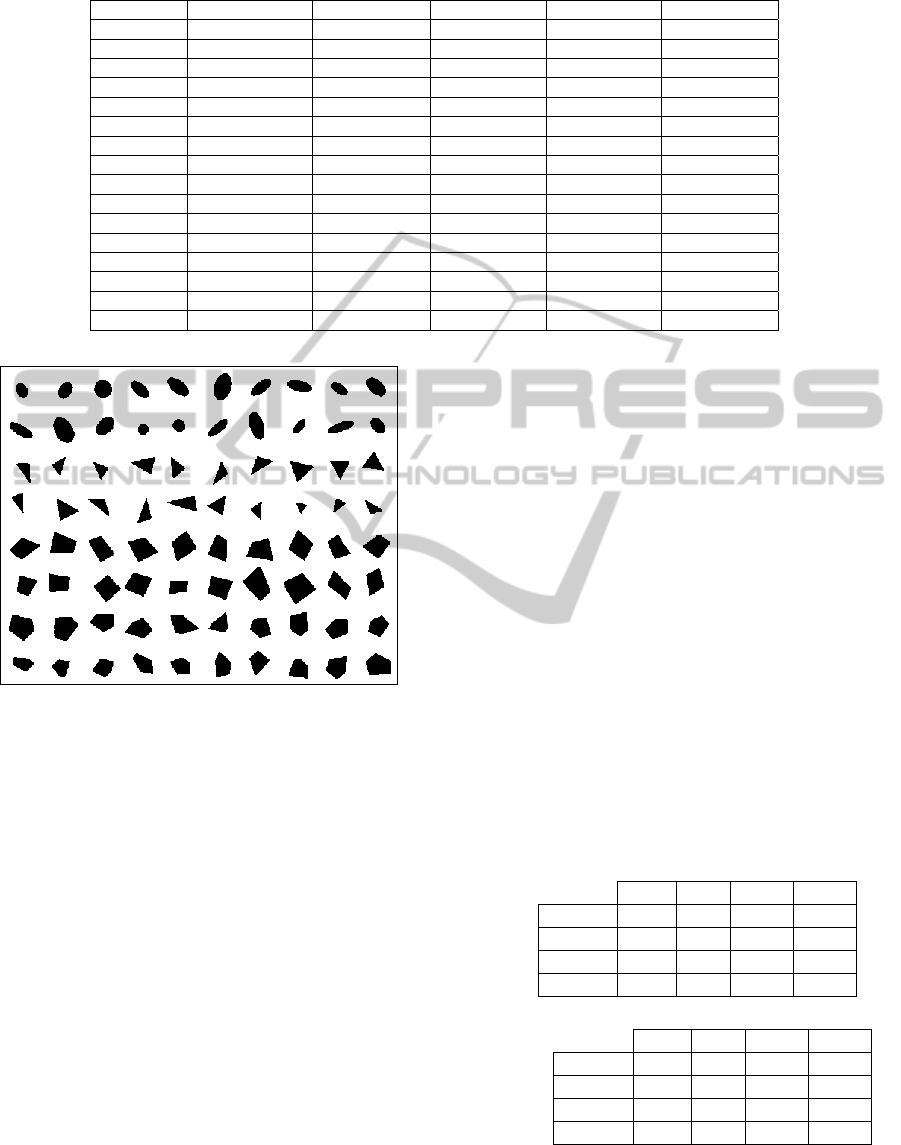
Table 1: Statistics of various features: minimum (min), maximum (max), average (mean), standard deviation (std).
Feature Type min max mean std
x
1
Continuous 1.701448 8.377751 4.454941 1.140443
x
2
Continuous 1.514297 7.804499 3.498672 1.045025
x
3
Continuous 0.696465 6.744747 2.885716 1.118037
x
4
Continuous 0.370465 5.971567 2.364773 1.044711
x
5
Continuous 0.310115 8.298036 2.304304 1.247915
x
6
Continuous 0.36461 7.128069 2.385969 1.128959
x
7
Continuous 0.592846 7.266519 2.739837 1.141935
x
8
Continuous 1.217079 7.53666 3.128944 1.004257
x
9
Continuous 2.013517 8.473231 4.342271 1.123421
x
10
Continuous 2.723593 9.918232 6.707424 1.092196
x
11
Continuous 2.448623 10.02286 7.068465 1.218173
x
12
Continuous 2.990693 10.25685 7.114858 1.231805
x
13
Continuous 2.971142 10.21713 7.099484 1.235933
x
14
Continuous 2.86403 10.07608 7.065576 1.224407
x
15
Continuous 2.970317 10.00546 6.88241 1.210681
x
16
Continuous 2.966 9.986865 6.524544 1.192905
Figure 3: Sample of geometric shapes in the adopted
dataset.
4.2 Experiments and Results
The proposed approach was tested on the adopted
benchmark dataset described in the previous
subsection. We built different RBF network models
using ring-wedge energy features extracted for each
shape in the dataset. This helps in reducing the
dimensionality of the vector space and handling
various shape deformations. We employed 5-fold
stratified cross validation to evaluate the quality of
the models. In this approach the dataset is randomly
split into 5 non-overlapping partitions (a.k.a. folds).
During this process, a stratified method is used to
ensure that the distribution of different categories of
the target variable is approximately the same in
various partitions. Then, a model is built using four
partitions (i.e. 80% of the dataset) for training and
evaluated on the remaining partition (1 out of 5
partitions, i.e. 20% of the dataset). This process is
repeated five times. Each time a different partition is
used for testing and the remaining four partitions for
training. The overall performance measures are
averaged over the 5 models.
The RBF network model uses the hybrid
learning algorithm which is implemented in the
DTREG software package as explained previously
in Section 3. The performance of RBF network
model is assessed in terms of a confusion matrix
which shows how each category is predicted by the
model. In all experiments, we assumed equal
misclassification costs for all categories. Table 2
shows the resulting confusion matrix for the RBF
network model for both training and testing datasets
using 5-fold stratified cross validation. The numbers
in the diagonals are the correctly classified cases for
each category whereas the off-diagonal cells
represent the misclassified cases.
Table 2: 5-fold stratified cross validation of RBF
classification model in terms of confusion matrix for (a)
Training and (b) Testing.
(a) Training Predicted Category
S1 S2 S3 S4
Actual
Category
S1 200 0 0 0
S2 0 200 0 0
S3 0 2 187 11
S4 0 0 1 199
(b) Testing
Predicted Category
S1 S2 S3 S4
Actual
Category
S1 200 0 0 0
S2 0 200 0 0
S3 0 2 180 18
S4 2 0 8 190
We then compared the performance of RBF
networks with two other standard classifier models:
multi-layer perceptron (MLP) neural networks and
CLASSIFICATION OF DEFORMABLE GEOMETRIC SHAPES - Using Radial-Basis Function Networks and
Ring-wedge Energy Features
359

decision trees (DTs). The constructed MLP is a 3-
layer neural network in which there are 16 neurons
in the input layer (number of features), 6 neurons in
the hidden layer with sigmoid activation functions,
and 4 neurons in the output layer (number of
categories of the target variable) with linear
activation functions. The input layer standardizes
each input variable so that its value falls in the range
between -1 and +1. The network weights are
adjusted using a conjugate gradient with line search
back-propagation algorithm. This algorithm
converges significantly faster than the original
gradient decent backpropagation developed by
Rumelhart and McClelland for MLP (Sherrod,
2011).
The constructed decision tree is a single binary
tree that shows how the target variable can be
predicted using values of a set of the predictor
variables. Each non-terminal (internal) node in the
decision tree splits a group of rows of the dataset
into two subgroups based on one particular predictor
variable. During the composition of the decision
tree, a recursive partitioning procedure uses Gini’s
criterion and backward pruning to build an optimal
size tree while maximizing the heterogeneity of the
categories of the target variable in the child nodes.
Table 3 shows the comparison results for the
constructed RBF, MLP and DT models in terms of
the misclassification rates (i.e. the percentage of
observations that are predicted to be of a category
different than the actual category associated with
them). We can clearly notice that the classification
error rate when using the RBF model is lower than
that for MLP and DT.
Table 3: Comparing misclassification rates for different
models.
Dataset
Method
RBF MLP DT
Training 1.75 4.5 6.625
Testing 3.75 5.25 17.0
To see how the constructed RBF model behaves
for each category as compared to other methods, we
used four other performance measures. These
measures are: sensitivity (Sn), specificity (Sp),
positive predictive value (PPV) and negative
predictive value (NPV). These values are assessed
for each category. We refer to a given category s
i
as
positive category and all other categories are
grouped and regarded as negative category for this
given category. To define performance measures
mathematically, let TP
i
, TN
i
, FP
i
, and FN
i
refer to
the number of true positive, number of true negative,
number of false positive and number of false
negative for category s
i
, respectively. Then the
evaluations of the performance measures are defined
as follows for category s
i
:
Sensitivity of s
i
: the proportion of those
predicted as being of category s
i
that are truly
predicted by the model.
/ ( ), 1, 2,..., .
iii i
Sn TP TP FN i S
=
+=
(9)
Specificity of s
i
: the proportion of those
predicted to be of categories other than s
i
that
are truly predicted by the model.
/ ( ), 1, 2,..., .
iiii
Sp TN TN FP i S
=
+=
(10)
PPV: the proportion of those who are actually
of category s
i
and are truly predicted by the
model.
/ ( ), 1, 2,..., .
iiii
PPV TP TP FP i S
=
+=
(11)
NPV: the proportion of those who are of
categories other than s
i
and are truly predicted
by the model.
/ ( ), 1, 2,..., .
iiii
NPV TN TN FN i S
=
+=
(12)
Table 4: The per-category performance comparison for
different models during training.
Cat. Measure
Method
RBF MLP DT
s
1
Sn 100 97 93
Sp 100 100 98.67
PPV 100 100 95.88
NPV 100 99.01 97.69
s
2
Sn 100 100 97
Sp 99.67 99.33 98.17
PPV 99.01 98.04 94.63
NPV 100 100 98.99
s
3
Sn 93.5 90.5 91
Sp 99.83 97.67 97.17
PPV 99.47 92.82 91.46
NPV 98.67 96.86 97
s
4
Sn 99.5 94.5 92.5
Sp 98.17 97 97.17
PPV 94.76 91.3 91.58
NPV 99.83 98.15 97.49
Tables 4 and 5 compare the per-category
performance measures for the three constructed
models for the training and testing datasets,
respectively. Again, the results demonstrate that the
RBF network model outperforms MLP and DT
models.
ICAART 2012 - International Conference on Agents and Artificial Intelligence
360

Table 5: The per-category performance comparison for
different models during testing.
Cat. Measure
Method
RBF MLP DT
s
1
Sn 100 98 86.5
Sp 99.67 99.83 95.83
PPV 99.01 99.49 87.37
NPV 100 99.34 95.51
s
2
Sn 100 100 89
Sp 99.67 99 96.5
PPV 99.01 97.09 89.45
NPV 100 100 96.34
s
3
Sn 90 87 79
Sp 98.67 97.5 92.67
PPV 95.74 92.06 78.22
NPV 96.24 95.74 92.98
s
4
Sn 95 94 77.5
Sp 97 96.67 92.33
PPV 91.35 90.38 77.11
NPV 98.31 94.1 92.49
5 CONCLUSIONS
In this paper we described a novel approach for
automatic classification of deformable geometric
shapes based on RBF networks and transform-based
features. The performance of the proposed system is
empirically evaluated and compared with other
classification algorithms. Results showed that the
proposed approach has better performance than the
other considered classification algorithms in terms
of classification accuracy, sensitivity, specificity,
positive predictive value, and negative predictive
value. As a future work we are comparing the
proposed approach with other classifiers and we are
investigating other ways to improve the results
further.
ACKNOWLEDGEMENTS
The authors would like to acknowledge the support
of the Intelligent Systems Research Group and
Deanship of Scientific Research at King Fahd
University of Petroleum and Minerals (KFUPM),
Dhahran, Saudi Arabia.
REFERENCES
Barutcuoglu, Z., DeCoro, C., 2006. Hierarchical shape
classification using Bayesian aggregation. In
Proceedings of the IEEE International Conference on
Shape Modeling and Applications, Matsushima, Japan.
Bishop, C. M., 1995. Neural networks for pattern
recognition, Oxford University Press, New York.
Chang, C. C., Hwang, S. M., Buehrer, D. J., 1991. A shape
recognition scheme based on relative distances of
feature points from the centroid. Pattern Recognition,
24(11): 1053–1063.
Chen, S., Hong X., Harris, C. J., 2005. Orthogonal
forward selection for constructing the radial basis
function network with tunable nodes. In Proceedings
of the IEEE International Conference on Intelligent
Computing.
Chen, L., Feris, R. S., Turk, M., 2008. Efficient partial
shape matching using Smith-Waterman algorithm. In
Workshop on Non-Rigid Shape Analysis and
Deformable Image Alignment (NORDIA'08), in
conjunction with CVPR'08, Anchorage, Alaska.
Chen, L., McAuley, J., Feris, R., Caetano, T., Turk, M.,
2009. Shape classification through structured learning
of matching measures. In Proceeding of the IEEE
Conference on Computer Vision and Pattern
Recognition (CVPR 2009), Miami, Florida.
Costa, L., Cesar Jr., R. M., 2000. Shape analysis and
classification: Theory and practice, CRC Press.
El-Alfy, E.-S. M., 2008. Abductive learning approach for
geometric shape recognition. In Proceedings of the
International Conference on Intelligent Systems and
Exhibition, Bahrain.
Lazzerini, B., Marceelloni, F., 2001. A fuzzy approach to
2-D shape recognition. IEEE Transactions on Fuzzy
Systems, 9(1): 5-16.
George, N., Wang, S., Venable, D. L., 1989. Pattern
recognition using the ring-wedge detector and neural
network software. SPIE, 1134: 96-106.
Gorelick, L., Galun, M., Sharon, E., Basri, R., Brandt, A.,
2006. Shape representation and classification using the
Poisson equation. IEEE Transactions on Pattern
Analysis and Machine Intelligence, 28(12): 1991-
2005.
Haykin, S., 2009. Neural networks and learning machines.
Third Edition, Prentice-Hall.
Ling, H., Jacobs, D. W., 2007. Shape classification using
the inner-distance. IEEE Transactions on Pattern
Analysis and Machine Intelligence, 29(2): 286-299.
McNeil, G., Vijayakumar, S., 2005. 2D shape
classification and retrieval. In Proceedings of the
International Joint Conference on Artificial
Intelligence (IJCAI’05), Edinburgh, Scotland.
Moorehead, L. B., Jones, R. A., 1988. A neural network
for shape recognition. In Proceedings of the IEEE
Region 5 Conference, Piscataway, NJ.
Neruda, R., Kudova, P., 2005. Learning methods for radial
basis functions networks. Future Generation
Computer Systems, 21: 1131-1142.
Powel, M., 1985. Radial-basis functions for multivariable
interpolation: A review. In Proceedings of the IMA
Conference on Algorithms for the Approximation of
Functions and Data, Shrivenham, England.
Pun, C.-M., Lin, C., 2010. Geometric invariant shape
classification using hidden Markov model. In
Proceedings of the IEEE International Conference on
Digital Image Computing: Techniques and
Applications (DICTA 2010).
CLASSIFICATION OF DEFORMABLE GEOMETRIC SHAPES - Using Radial-Basis Function Networks and
Ring-wedge Energy Features
361

Sherrod, P. H., 2011. DTREG: Predictive modeling
software. http://www.dtreg.com/DTREG.pdf
Super, B. J., 2004. Fast correspondence-based system for
shape retrieval. Pattern Recognition Letters, 25: 217-
225.
Tsai, A., Wells, W. M., Warfield, S. K., Willsky, A. S.,
2005. An EM algorithm for shape classification based
on level sets. Medical Image Analysis, 9: 491-502.
Yau, H-C., 1990. Transform-based shape recognition
employing neural networks. Ph.D. Dissertation,
University of Texas at Arlington.
Yau, H.-C., Manry, M. T., 1991. Shape recognition with
nearest neighbor isomorphic network. In Proceedings
of the IEEE-SP Workshop on Neural Networks for
Signal Processing, Princeton, NJ.
Yau, H.-C., Manry, M. T., 1991. Iterative improvement of
a nearest neighbor classifier. Neural Networks, 4: 517-
524.
Zhang, J., Zhang, X., Krim, H., Walter, G. G., 2003.
Object representation and recognition in shape spaces.
Pattern Recognition, 36: 1143-1154.
ICAART 2012 - International Conference on Agents and Artificial Intelligence
362
