TRAINING RADIAL BASIS FUNCTION NETWORKS

BY GENETIC ALGORITHMS

Juliano F. da Mota

1,3

, Paulo H. Siqueira

2,3

, Luzia V. de Souza

2,3

and Adriano Vitor

1,3

Department of Mathematics, Paraná State University, Com. Norberto Marcondes Avenue 733, Campo Mourão, Brazil

Department of Graphical Expression, Paraná Federal University, Cel Francisco H. dos Santos Avenue, Curitiba, Brazil

Graduate Program in Numerical Methods in Engineering, Paraná Federal University, Curitiba, Brazil

Keywords:

Radial basis function neural networks, Evolutionary computation, Pattern classiﬁcation.

Abstract:

One of the issues of modeling a RBFNN - Radial Basis Function Neural Network consists of determining the

weights of the output layer, usually represented by a rectangular matrix. The inconvenient characteristic at

this stage it’s the calculation of the pseudo-inverse of the activation values matrix. This operation may become

computationally expensive and cause rounding errors when the amount of variables is large or the activation

values form an ill-conditioned matrix so that the model can misclassify the patterns. In our research, Genetic

Algorithms for continuous variables determines the weights of the output layer of a RBNN and we’ve made

a comparsion with the traditional method of pseudo-inversion. The proposed approach generates matrices of

random normally distributed weights which are individuals of the population and applies the Michalewicz’s

genetic operators until some stopping criteria is reached. We’ve tested four classiﬁcation patterns databases

and an overall mean accuracy lies in the range 91–98%, in the best case and 58–63%, in the worse case.

1 INTRODUCTION

For a long time scientists have been trying to develop

methods for pattern classiﬁcation problems wich may

help a decision taker in a uncertain scenario. Several

mathematical and statistical methods had been devel-

oped and, for this reason, improvements in existents

methods and the building up of new methods wich

may reduce the computational effort, offer better re-

sults or both are required nowadays.

Every single existent method offer a different op-

tion relative to speed and quality of the prediction or

classiﬁcation. The most difﬁcult task, wich every re-

searcher yearns, is to develop a method capable of get

a high accuracy in a minimal time given the need for

speed of the on-line era. By “high accuracy” we mean

an error as small as possible and a correct classiﬁed

percentual as big as possible, considering a pattern

classiﬁcation problem.

This study compares two training methods of a

RBFNN, one of them is considered traditional, which

is based in calculating the pseudo-inversion of a rect-

angular matrix and the other uses genetic algorithms

for continuous data, changing this matrix into a ge-

netic population individual, and the main objective is

to ﬁnd the optimal (or near-optimal) matrix through

natural selection and genetic operators.

To reach this goal, the basic precepts of Radial

Basis Function Neural Networks and Genetic Algo-

rithms are presented and its main features are ex-

plained in order to form a conceptual basis for the

experiments.

2 SOME RELATED

RESEARCHES

Trying to solve the main problem of the classical ap-

proach of training a RBFNN, which is the need to

calculate the pseudoinverse of a rectangular matrix,

some authors have proposed alternative methodolo-

gies to change that problem into another of lower

computational complexity.

The researchers (Li and Ling, 2011) applied the

idea of getting the weights of the hidden layer of a

RBFNN to develop a generalized model predictive

control in a power generating unit that had two in-

put and two output variables. The experiment was to

compare the performance of the proposed algorithm

(called GA-RBF) with the performance of a Multi-

layer Perceptron using the back-propagation training

373

F. da Mota J., H. Siqueira P., V. de Souza L. and Vitor A..

TRAINING RADIAL BASIS FUNCTION NETWORKS BY GENETIC ALGORITHMS.

DOI: 10.5220/0003751903730379

In Proceedings of the 4th International Conference on Agents and Artiﬁcial Intelligence (ICAART-2012), pages 373-379

ISBN: 978-989-8425-95-9

 2012 SCITEPRESS (Science and Technology Publications, Lda.)

algorithm. The proposed technique has a mean square

error of the order of 10

−5

, while the Perceptron tested

missed about 10

−1

The research of (Changbing and Wei, 2010) ap-

plied RBFNN trained by GA to forecast the risk in

an aquatic environment. The tests show that the pro-

posed model outperformed the "gray model" which

uses a ﬁrst order differential equation to estimate val-

ues based on historical data. There are charts on

which you can visualize the superiority of the pro-

posed model to predict the risk.

By the other hand (Ming et al., 2010) applied the

same basic idea for predicting the ﬂow in a network.

The results of the experiment, in which the ﬂow of

a network with 40 points was predicted, show that

the relative error in the prediction of a RBFNN train-

ing via the pseudo-inversion (traditional) was 0.0247

while the RBFNN trained by GA could miss only

0.0177, a reduction of almost 30% in error.

The research (Kurban and Be¸sdok, 2009) com-

pared four algorithms to train a RBFNN: Bee Colony,

GA, Kalman ﬁlter and gradient descent. They tested

three databases available in (Frank and Asuncion,

2010) and one database application proposed by the

authors. In all of tested datasets the Bee Cllony algo-

rithm performances was slightly higher than the GA,

both featuring an accuracy above 90% accuracy the

test set in the database in (Frank and Asuncion, 2010)

and over 70% of the database application in sensors

proposed by the authors.

3 RADIAL BASIS FUNCTION

NEURAL NETWORKS

A RBFNN is feed-forward and it has only two layers,

one of them is a hidden layer and the other is the out-

put layer. In the hidden layer the activation functions

of neurons are radial basis functions. A RBF - Ra-

dial Basis Function is deﬁned by (Haykin, 2001) as

any function that its functional values are equal to the

norm of its arguments.

3.1 Neural Networks wich uses Radial

Basis Functions

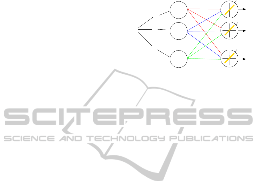
The learning process of this network has its founda-

tions in the theory of nonlinear programming. The ar-

chitecture of a RBFNN is quite simple, there are only

two layers in addition to the input nodes, one hidden

layer, which has radial basis functions as activation

functions and an output layer which has linear func-

tions as activation, as seen in Figure 1.

Figure 1: Representation of the Architecture of a RBFNN.

Each neuron in the hidden layer has an associated

vector, called the center of the neuron, which deﬁnes

the center of the receptive ﬁeld of that neuron. Gen-

erally such vectors are stored in a C matrix, called the

matrix of centers of neurons. These vectors have a

strong inﬂuence on network performance. Later, in

section 3.2 some methods will be brieﬂy presented.

The m-th activation value from a hidden layer neu-

ron depends of the distance between the input node x

and the center c

, where c

∈ C is the center of the

m-th neuron. Thus, by the classical approach, train a

RBFNN is equivalent to calculate the wheights matrix

w to ﬁt each y to one target t, as shows the equation 1,

= w

∑

k=1



||x

−C||



. (1)

3.2 Neurons Centers Selection

The task of selecting the neurons centers is essentially

a clustering problem. There are a few classic strate-

gies described in (Haykin, 2001) and a brief discus-

sion of these strategies is presented below.

3.2.1 Random Fixed Centers

This is the simplest and least expensive way to se-

lect the centers. Although simple, it is considered by

(Haykin, 2001) as “the most sensible approach” be-

cause in each experiment a different part of the ma-

trix of observations is used, and for this reason, the C

matrix will contain a good representation of the data

space.

The limitation of this method lies in the need of

a large training set to achieve a satisfactory perfor-

mance. Possibly, the standard most commonly used

training 60–20–20, meaning 60% for the training set

and 20% validation and testing, would probably have

to be modiﬁed and hence the model could lose the

ability to generalize.

ICAART 2012 - International Conference on Agents and Artificial Intelligence

374

3.2.2 Self-organized Selection of Centers

Also described in (Haykin, 2001) and (Silva et al.,

2010), this method consists of the main idea of the

SOM - Self Organizing Map Algorithm proposed by

Kohonen apud (Haykin, 2001), wich is described be-

low:

1. Choose distinct random values as initial centers,

in most cases elements of the training set;

2. During the n-th iteration, take a sample of training

set;

3. Find the center with the minimal euclidian dis-

tance to each entering vector;

4. Update the winner center position acording the

equation:

c(new) = c(old) + η(x− c) (2)

where η ∈ (0, 1) is a learning rate, x is the entering

vector and c is the winner center.

5. Back to Step 2 until no noticiable changes in the

centers matrix can be perceived.

The main difference between this algorithm and

the classical SOM algorithm is precisely the absence

of a neurons map, i.e., no neighborhood is consid-

ered to update the neurons. That means to say a SOM

with the "Winner Takes All" principle (Siqueira et al.,

2005). where only the winner neuron is updated.

3.2.3 Supervisioned Selection of Centers

This is the most generic form to make the selection of

centers. The idea is to ﬁt the centers by error correc-

tion and thus RBFNN resembles the classical Percep-

tron.

4 CONTINUOUS DATA GENETIC

ALGORITHMS

The GA - Genetic Algorithm as described in (Hol-

land, 1975) apud (Man et al., 1996) are basically a set

of algorithms based on the principles of evolutionary

biology stated by Charles Darwin in his book known

worldwide The Evolution of Species. The main objec-

tive of the GAs is to optimize functions.

The considered principles in a GA preparation are

natural selection, heredity, mutation and recombina-

tion (crossing-over). When translating into a math-

ematical language, these principles become genetic

operators of crossover and mutation, such a way that

heritability and natural selection becomes a decision

rule.

The basic algorithm, systematized by (Holland,

1975) apud (Man et al., 1996), has low implemen-

tation complexity and this is one of the great advan-

tages of this technique. The steps of the algorithm are

described in the algorithm in Figure 2.

It is noteworthy that, initially, the binary number

base (binary representation) is considered for imple-

mentation and application of GAs. Today, however,

is quite common to ﬁnd applications where the dec-

imal number base is used. Possibly, this change has

been due to real representation allow greater range of

operators, as will be shown in section 4.1.

Let g = 0 the generation counter;

Create and initialize a presized population;

while no stop criteria is reached do;

Evaluate the ﬁtness of each individual in population;

Perform reproduction to generate offspring;

Select the new population;

Advance to the new generation, i. e., g = g+ 1;

end while

Figure 2: The GA Algorithm.

4.1 Real Representation and

Michalewicz Operators

One of the studies using the real representation can

be found in (Michalewicz et al., 1994), were there

are three crossover operators and three mutation op-

erators described and mathematically justiﬁed. Ad-

ditionally to those descriptions, we describe also an

extra mutation operator. In all operators, p

are the

parents and c

are the offspring.

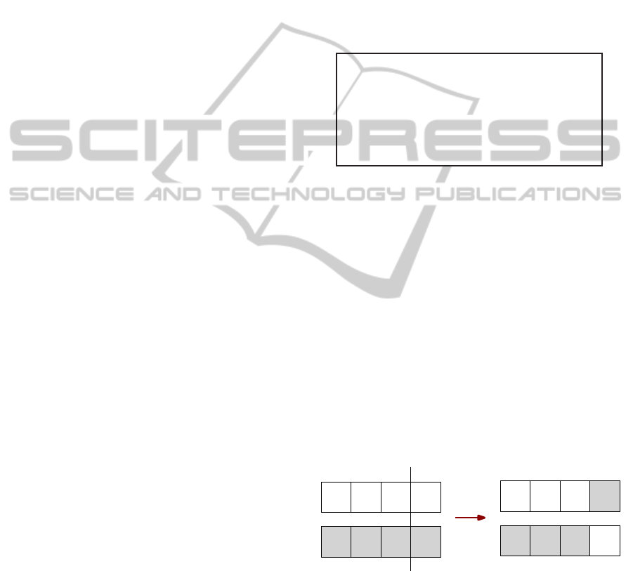
The ordinary crossover is a variation of a conven-

tional one point crossover, which is used in the binary

representation, adapted to the real representation, as

we can see in Figure 3.

1,5 9,2

31,2

6,8

0,8

7,4

1,3

5,7

1,5

9,2

31,2

6,80,8

7,4

1,3

5,7

Parents Oﬀspring

Figure 3: One Point Crossover Representation.

Given two individuals, the arithmetical crossover

generates,

= βp

+ (1− β)p

and

= βp

+ (1− β)p

with β ∼ U(0, 1).

For another two individuals such that the ﬁtness of p

is greater than the ﬁtness of p

, the heuristic crossover

TRAINING RADIAL BASIS FUNCTION NETWORKS BY GENETIC ALGORITHMS

375

generates,

c = p

+ β(p

− p

) where β ∼ U(0, 1).

Given an individual p, the uniform mutation oper-

ator replaces one gene by a random number coming

from a uniform distribution, i.e.,



U(a

, b

), if i = j

, otherwise.

The values a

and b

represents the interval limits

to the individual c

, just in case of a factibility restric-

tion.

Given an individual p, the limit mutation operator

replaces one gene by one of the interval limits [a

, b

avoiding the arithmetical crossover to take the genes

to the interval center, here we consider r ∼ U(0, 1),







, if r < 0, 5 and i = j

, if r > 0, 5 e i = j

, otherwise .

Finally, an individual p, the non-uniform mutation

operator replaces one gene by a random number com-

ing from a non-uniform distribution, i.e.,







+ (b

− p

) f(G), if r

< 0, 5 and i = j

− (p

− a

) f(G), if r

≥ 0, 5 and i = j

, otherwise .

considering,

f(G) =





1−

max



where G is the current generation, G

max

is the maxi-

mum number of generations and r

, r

∼ U(0, 1). The

application of non-uniform mutation in all genes of

this individual is called multiple non-uniform muta-

tion.

5 EXPERIMENTS AND RESULTS

ANALYSIS

In our experiments, the performance of a RBFNN us-

ing the traditional method of training, the pseudo-

inversion of the matrix that contains the activa-

tion values of the intermediate layer, was com-

pared with alternative training pathway GA, con-

sidering Michalewicz operators (Michalewicz et al.,

1994). We’ve used the already well-known classiﬁ-

cation problems - Iris, Contraceptive Method Choice

(CMC), Cancer and Blood Transfusion (BT) - data

sets that are found in (Frank and Asuncion, 2010).

The characteristics of the sets used in the tests are

Table 1: Datasets Features.

Dataset Entries Outputs Training Validation Test

Iris 4 3 90 30 30

CMC 9 3 884 295 294

Cancer 9 2 420 140 139

BT 4 2 449 150 149

shown in Table 1, the number of variables in standard

input, output and the number of patterns in each set.

For all data sets, we performed an experiment that

consisted of ﬁve steps:

1. Separate the database into three sets:

• Training set, with 60% of the examples;

• Validation set, with 20% of the examples and;

• Set of tests, with 20% of the examples.

2. Train a RBFNN 100 epochs with each approach

(pseudo-inversion and GA) and obtain CCP - Cor-

rect Classiﬁed Percentage in each set of item 1,

especially set of tests;

3. Record the results of the statistical percentages of

correct classiﬁcations of the two training meth-

ods;

4. Considering a signiﬁcance level of 5% to test the

hypothesis of equality of variances in order to

determine which test comparing the means used,

writing H = 0 if variances are equal and H = 1

otherwise;

5. Considering a signiﬁcance level of 5%, perform

two comparison tests medium with the following

assumptions:

First Test Second Test

: Average PI = Average GA h

: Average PI = Average GA

: Average PI > Average GA h

: Average PI < Average GA

considering h

= 0 if h

is not rejected in the ﬁrst test

and h

= 1, oterwise. Considering yet h

= 0 if h

not rejected in the second test and h

= 1, otherwise.

According to the literature, one of the most im-

portant parameters for a neural network, including the

RBFNN, is the number of neurons in its layers, in the

speciﬁc case of this research, the amount of interme-

diate layer neurons. The limit here is set to test from

two to 10 neurons, increasing of two at each experi-

ment.

Two other major issues, when talking about the

parameters of a RBFNN, are the method of centers se-

lection and the deﬁnition of the spread of the Gaussian

activation functions in the hidden layer. The method

of centers selection used in this study was the self-

organized selection of centers, described in Section

3.2.2 and the method for setting the spread of each

RBF is described in (Silva et al., 2010) and basically

ICAART 2012 - International Conference on Agents and Artificial Intelligence

376

consists into calculating the radius of each function

based on the mean square distance between the inputs

and the centers of the neurons that received an update

during the self-organized selection of centers.

The parameters selection of a GA also does not

have a consolidated method, varying according to

each application. Therefore, it is necessary to perform

some initial tests to observe the inﬂuence of each pa-

rameter in the performance of the algorithm. In this

research, we’ve made more than 50 preliminary tests

and the best parameter setting is in Table 2.

Table 2: GA Parameters.

Parameter Value

Initial Population 100

Probability Crossing Operators 80%

Probability Mutation Operators 10%

Maximum Number of Generations 100

Talking about the mutation operators wich have

restricted the range to the generated numbers, i. e.,

the Limit Mutation, Non-uniform Mutation and Non-

uniform Multiple Mutation, the range adopted in all

cases was to accept an increase of up to 100% of the

highest absolute value of a gene in any individual.

This means that if the highest absolute value

among the genes of all individuals is τ, then the possi-

ble range for the generation of a mutation gene would

be (−2 · τ, 2 · τ). This measure sought a balance be-

tween excessiveextrapolation/restriction of the search

space.

In addition, with respect to the size of the initial

population we tested several initial population sizes

and the best result was obtained by the size of 100.

Although Genetic Algorithms are known for provid-

ing approximate solutions, here it’s being used as a

optimal solution pursuing technique.

The statistical results of 100 rounds for each data

set are in the Table 3–6, for Iris, CMC, Cancer and

BT, respectively. In the tables you can see informa-

tion about the mean and standard deviation of the per-

formance of each algorithm for each data set. In the

tables, the variable “NNeuro” represents the number

of neurons in the hidden layer. For each number of

neurons in the ﬁrst line depicts the statistics using

pseudo-inversion and the second statistics by the GA

approach.

As shown in Table 3, the proposed model using

GA to obtain the weight matrix showed a slightly

greater variability than the approach via pseudo-

inversion. The mean CCP by the GA approach was

not superior to the pseudo-inversion in any case and

according to the test t, for comparison between two

means, there was a tie with two neurons and superi-

ority of the approach via pseudo-inversion with other

amounts of neurons tested, notice that in all tests the

considered signiﬁcance level is 5 %.

Table 3: Results of Iris Set.

NNeuro Average±Std Dev Min Max H h

90, 5%± 5, 6% 73,3% 100%

1 0 0

88, 4%± 7, 8% 63,3% 100%

92, 3%± 5% 73,3% 100%

1 1 0

87, 3%± 7% 66,7% 96,7%

93, 9%± 3, 9% 86,7% 100%

1 1 0

88, 7%± 5, 6% 73,3% 100%

94, 6%± 3, 8% 83,3% 100%

1 1 0

87, 1%± 7, 3% 70% 100%

94, 6%± 3, 8% 86,7% 100%

1 1 0

85, 2%± 8, 1% 63,3% 100%

The results in Table 4 shows that considering a

signiﬁcance level of 5%, the variance of the perfor-

mances of both techniques is not statistically sig-

niﬁcant and there is superiority of the approach via

pseudo-inversion in two cases: six and 10 neurons in

the hidden layer, given the values of h

. Even compar-

ing the best performance in both cases, the approach

via GA was inferior about two percentage points ap-

proximately.

Table 4: Results of Contraceptive Method Choice Set.

NNeuro Average±Std Dev Min Max H h

57%± 2, 7% 49% 63,3%

0 0 0

56, 7%± 2, 9% 49% 63,3%

57, 1%± 2, 2% 52,7% 61,2%

0 0 0

56, 7%± 2, 6% 50,7% 62,6%

58, 5%± 3, 3% 51,7% 67,7%

0 1 0

56, 9%± 3, 2% 49,7% 64,3%

58, 2%± 3, 2% 50,7% 65,6%

0 0 0

57, 1%± 3, 2% 48,6% 62,9%

60, 5%± 2, 8% 52% 65%

0 1 0

58, 4%± 2, 7% 51,4% 64%

For the Cancer dataset in Table 5, considering a

signiﬁcance level of 5%, there was no difference be-

tween the performance variances of both techniques,

except with 10 neurons, and that the only case in

which there was a statistically signiﬁcant difference,

with six neurons in the hidden layer, this case was fa-

vorable to the GA approach given the h

value.

Finally, in Table 6 considering 5% of signiﬁcance,

there was no difference between the variances of the

performance and the pseudo-inversion approach was

better in three of ﬁve numbers of neurons tested: six,

eight and 10 neurons. Once the volume of two four

neurons there was a tie.

TRAINING RADIAL BASIS FUNCTION NETWORKS BY GENETIC ALGORITHMS

377

Table 5: Results for the Cancer Dataset.

NNeuro Average± Std Dev Min Max H h

95, 6%± 1, 5% 92,1% 98,6%

0 0 0

96%± 1, 5% 92,9% 98,6%

95, 3%± 1, 7% 92,1% 98,6%

0 0 0

95, 9%± 1, 4% 92,9% 98,6%

95, 1%± 1, 7% 90,7% 97,9%

0 0 1

96%± 1, 6% 92,1% 98,6%

96%± 1, 2% 94,3% 98,6%

0 0 0

96, 3%± 1, 3% 93,6% 98,6%

95, 8%± 1, 6% 92,1% 100%

1 0 0

96, 2%± 1, 4% 93,6% 99,3%

Table 6: Results for Blood Transfusion Dataset.

NNeuro Average± Std Dev Min Max H h

75, 9%± 3, 2% 68,5% 83,9%

0 0 0

75, 9%± 3, 2% 68,5% 83,9%

77, 7%± 3, 3% 70,5% 84,6%

0 0 0

77, 2%± 3, 2% 71,1% 85,2%

78, 8%± 3, 9% 67,8% 89,3%

0 1 0

77, 5%± 3, 4% 67,8% 85,2%

77, 5%± 2, 4% 71,1% 81,9%

0 1 0

75, 9%± 3% 67,8% 81,9%

77, 6%± 3, 5% 71,8% 85,2%

0 1 0

76%± 3, 5% 68,5% 84,6%

6 CONSIDERATIONS AND

FUTURE WORK

Considering the results obtained and previously dis-

cussed, we can say that:

• the genetic operators presented did not produced

good populations, given that the GA approach did

not overcome the traditional approach, except in

one case that can be seen in Table 5;

• the GA approach performance did not reach the

expectations when compared with the traditional

approach, because even in the situation was better,

this superiority was not unquestionable;

• there were two cases where none of the two ap-

proaches achieved a signiﬁcant result: in the data

set “Contraceptive Method Choice”, the best per-

formances of both algorithms was below 70% on

all executions and below 60% on average. In the

case of the “Blood Transfusion”, despite the mean

CCP was higher 70%, a possible application in

reality would not be feasible because the model

would not be reliable;

• the training via GA produced results lower than

the pseudo-inversion in three of four sets tested,

considering the signiﬁcance deﬁned in the tests.

Taking an overview of the results, considering a

5% level of signiﬁcance, we can say that the GA ap-

proach even being able to produce results as good

as the supposedly exact approach had a signiﬁcantly

lower performance in the databases we’ve tested.

However, it is necessary to consider that the exact ap-

proach suffers with complexity and numerical round-

ing errors with the growth of the number of neurons in

the hidden layer. Thus, taking into account the adapt-

ability of GA, if new more robust genetic operators

are developed will overcome this limitation.

6.1 Future Works

Noting the apparent failure of the considerations

made in this study, below we’ve listed some possi-

ble suggestions for future works that may continue or

refute this line of thinking:

• test other GA operators;

• compare other search algorithms (and GA) with

the pseudo-inversion approach;

• compare other search algorithms with supervised

learning approach;

• use statistical techniques such as Principal Com-

ponent Analysis and Fator Analysis in the treat-

ment of data in order to see if they can help im-

prove performance in sets with similar character-

istics o the "Contraceptive Method Choice ", in

which both approaches had less than 70% perfor-

mance.

REFERENCES

Changbing, L. and Wei, H. (2010). Application of genetic

algorithm-rbf neural network in water environment

risk prediction. 2nd International Conference on

Computer Engineering and Technology 2010, pages

239–242.

Frank, A. and Asuncion, A. (2010). Uci machine learning

repository.

Haykin, S. (2001). Redes neurais - princípios e práticas.

Bookman.

Holland, J. (1975). Adaption in Natural and Artiﬁcial Sys-

tems. MIT Press.

Kurban, T. and Be¸sdok, E. (2009). A comparsion of rbf

neural netowrk training algorithms for inertial sen-

sor based terrian classiﬁcation. Sensors, pages 6312–

6329.

Li, N. and Ling, H. (2011). Study of an algorithm of ga-

rbf neural network generalized predictive control for

generating unit. International Conference on Elec-

tric Information and Control Engineering 2011, pages

1723–1726.

Man, K., Tang, K., and Kwong, S. (1996). Genetic algo-

rithms: concepts and applications. IEEE Transactions

on Industrial Electronics, 43(5):519–534.

ICAART 2012 - International Conference on Agents and Artificial Intelligence

378

Michalewicz, Z., Logan, T. D., and Swaminathan, S.

(1994). Evolutionary operators for continuous con-

vex parameter spaces. Proceedings of the 3rd Annual

Conference on Evolutionary Programming, pages 84–

97.

Ming, Z. Y., Bin, Z. Y., and Zhong, L. L. (2010). Appli-

cation of genetic algorithm and rbf neural network in

network ﬂow prediction. 3rd IEEE International Con-

ference on Computer Science and Information Tech-

nology 2010, pages 298–301.

Silva, I. N., Spatti, D. H., and Flauzino, R. A. (2010). Redes

neurais artiﬁciais - para engenharia e ciências apli-

cadas. Artliber.

Siqueira, P., Scheer, S., and Steiner, M. T. A. (2005). Ap-

plication of the "winner takes all" principle in wang’s

recurrent neural network for the assignment problem.

Lecture Notes in Computer Science, 3496(1):731–

738.

TRAINING RADIAL BASIS FUNCTION NETWORKS BY GENETIC ALGORITHMS

379