
STRATEGIES FOR CHALLENGING TWO-PLAYER GAMES
Some Lessons from Iterated Traveler’s Dilemma
Predrag T. To
ˇ
si
´
c
1
and Philip C. Dasler
1,2
1
Department of Computer Science, University of Houston, Houston, Texas, U.S.A.
2
Department of Computer Science, University of Maryland, College Park, Maryland, U.S.A.
Keywords:
Algorithmic game theory, Economic models of individual rationality, Strategic multi-agent encounters,
Non-zero-sum two-player games, Iterated games, tournaments, Performance analysis.
Abstract:
We study the iterated version of the Traveler’s Dilemma (TD). TD is a two-player, non-zero sum game that
offers plenty of incentives for cooperation. Our goal is to gain deeper understanding of iterated two-player
games whose structures are far from zero-sum. Our experimental study and analysis of Iterated TD is based on
a round-robin tournament we have recently designed, implemented and analyzed. This tournament involves 38
distinct participating strategies, and is motivated by the seminal work by Axelrod et al. on Iterated Prisoners
Dilemma. We first motivate and define the strategies competing in our tournament, followed by a summary
of the tournament results with respect to individual strategies. We then extend the performance comparison-
and-contrast of individual strategies in the tournament, and carefully analyze how groups of closely related
strategies perform when each such group is viewed as a “team”. We draw some interesting lessons from the
analyzes of individual and team performances, and outline some promising directions for future work.
1 INTRODUCTION
Game theory is important to AI and multi-agent
systems research communities because it provides
mathematical foundations for modeling interactions
among self-interested rational agents that may need
to combine competition and cooperation with each
other in order to meet their individual objectives (Par-
sons and Wooldridge, 2002; Rosenschein and Zlotkin,
1994; Wooldridge, 2009). An example of such inter-
actions is the iterated Prisoner’s Dilemma (PD) (Ax-
elrod, 1980; Axelrod, 1981), a classical two-person
non-zero-sum game that has been extensively studied
by psychologists, sociologists, economists, political
scientists, applied mathematicians and computer sci-
entists.
We study an interesting and rather complex 2-
player non-zero sum game, the (Iterated) Traveler’s
Dilemma (Becker et al., 2005; Capra et al., 1999;
Land et al., 2008; Pace, 2009). In TD, each player has
a large number of possible actions or moves. In the
iterated context, many possible actions per round im-
ply, for games of many rounds, an astronomic number
of possible strategies overall. We are interested in the
Iterated TD because its structure defies the usual pre-
scriptions of the classical game theory insofar as what
constitutes good or “optimal” play. We attempt to
gain a deeper understanding into what general types
of strategies can be expected to do well in an Iter-
ated TD setting via an experimental, simulation-based
study of several broad classes of strategies matched
against each other, that is, via a tournament. More-
over, we do so in a manner that, we argue, minimizes
the impact of individual parameter choices in those
strategies, thus enabling us to draw some broader,
more general conclusions.
The paper is organized as follows. We first define
the Traveler’s Dilemma, motivate its significance and
summarize the most relevant prior art. We then pur-
sue a detailed analysis of the “baseline” variant of the
game. Our analysis is based on a round-robin, many-
round tournament that we have recently designed, im-
plemented and run. We first summarize our main
findings on the relative performances of various in-
dividual strategies with respect to the “bottom line”
metric (which is, essentially, the appropriately nor-
malized total dollar amount won). We subsequently
focus on team performances of several carefully se-
lected groups of closely related strategies. We draw
a number of interesting conclusions based on our ex-
tensive experimentation and analyzes of the individ-
ual and team performances. Finally, we outline some
72
T. Toši
´
c P. and C. Dasler P..
STRATEGIES FOR CHALLENGING TWO-PLAYER GAMES - Some Lessons from Iterated Traveler’s Dilemma.
DOI: 10.5220/0003753900720082
In Proceedings of the 4th International Conference on Agents and Artificial Intelligence (ICAART-2012), pages 72-82
ISBN: 978-989-8425-96-6
Copyright
c
2012 SCITEPRESS (Science and Technology Publications, Lda.)

promising ways forward in this quest for deeper in-
sights into what we have informally dubbed the “far-
from-zero-sum” iterated two-player games.
2 TRAVELER’S DILEMMA
Traveler’s Dilemma was originally introduced in
(Basu, 1994). The motivation behind the game was
to expose some fundamental limitations of the classi-
cal game theory (Neumann and Morgenstern, 1944),
and in particular the notions of individual rational-
ity that stem from game-theoretic notions of “optimal
play” based on Nash equilibria (Basu, 1994; Basu,
2007; Wooldridge, 2009). The original version of
TD, which we will treat as the “default” variant of
this game, is defined as follows:
An airline loses two suitcases belonging to two
different travelers. Both suitcases happen to be iden-
tical and contain identical items. The airline is li-
able for a maximum of $100 per suitcase. The two
travelers are separated so that they cannot communi-
cate with each other, and asked to declare the value
of their lost suitcase and write down (i.e., bid) a value
between $2 and $100. If both claim the same value,
the airline will reimburse each traveler the declared
amount. However, if one traveler declares a smaller
value than the other, this smaller number will be taken
as the true dollar valuation, and each traveler will
receive that amount along with a bonus/malus: $2
extra will be paid to the traveler who declared the
lower value and a $2 deduction will be taken from the
person who bid the higher amount. So, what value
should a rational traveler (who wants to maximize the
amount she is reimbursed) declare?
A tacit assumption in the default formulation of
TD is that the bids have to be integers. That is, the
bid granularity is $1, as this amount is the smallest
possible difference between two non-equal bids.
This default TD game has some very interest-
ing properties. The game’s unique Nash equilibrium
(NE), the action pair (p, q) = ($2, $2), is actually
rather bad for both players, under the usual assump-
tion that the level of the players’ well-being is propor-
tional to the dollar amount they individually receive.
The choice of actions corresponding to NE results in
a very low payoff for each player. The NE actions
also minimize social welfare, which for us is simply
the sum of the two players’ individual payoffs. How-
ever, it has been argued (Basu, 1994; Capra et al.,
1999; Goeree and Holt, 2001) that a perfectly ratio-
nal player, according to classical game theory, would
“reason through” and converge to choosing the low-
est possible value, $2. Given that the TD game is
symmetric, each player would reason along the same
lines and, once selecting $2, would not deviate from it
(since unilaterally deviating from a Nash equilibrium
presumably can be expected to result in decreasing
one’s own payoff). In contrast, the non-equilibrium
pair of strategies ($100, $100) results in each player
earning $100, very near the best possible individual
payoff for each player. Hence, the early studies of TD
concluded that this game demonstrates a woeful inad-
equacy of the classical game theory, based on Nash
(or similar notions of) equilibria (Basu, 2007). Inter-
estingly, it has been experimentally shown that hu-
mans (both game theory experts and laymen) tend
to play far from the TD’s only equilibrium, at or
close to the maximum possible bid, and therefore fare
much better than if they followed the classical game-
theoretic approach (Becker et al., 2005).
We note that adopting one of the alternative con-
cepts of game equilibria found in the “mainstream”
literature does not appear to help, either. For example,
it is argued in (Land et al., 2008) that the action pair
($2, $2) is also the game’s only evolutionary equilib-
rium. Similarly, seeking sub-game perfect equilibria
(SGPE) (Osborne, 2004) of Iterated TD also isn’t par-
ticularly promising, since the set of a game’s SGPEs
is a subset of that game’s full set of Nash equilibria in
the mixed strategies.
We also note that the game’s only stable strategy
pair is nowhere close to being Pareto optimal: there
are many obvious ways of making both players much
better off than if they play the NE strategies. In par-
ticular, while neither stable nor an equilibrium in any
sense of those terms, ($100, $100) is the unique strat-
egy pair that maximizes social welfare and is, in par-
ticular, Pareto optimal.
3 ITERATED TD TOURNAMENT
Our Iterated Traveler’s Dilemma tournament has been
inspired by, and is in form similar to, Axelrod’s
Iterated Prisoner’s Dilemma tournament (Axelrod,
2006). In particular, it is a round-robin tournament
where each strategy plays against every other strategy
as follows: each agent plays N matches against each
other agent, incl. one’s own “twin”. A match con-
sists of T rounds. The agents do not know T or N and
cannot tweak their strategies with respect to the dura-
tion of the encounter. Similarly, the strategies are not
allowed to use any other assumptions (such as, e.g.,
the general or specific nature of the opponent they are
playing against in a given match). Indeed, the only
data available to the learning and adaptable strate-
gies in our “pool” of tournament participants (see be-
STRATEGIES FOR CHALLENGING TWO-PLAYER GAMES - Some Lessons from Iterated Traveler's Dilemma
73

low) is what they can learn and infer about the future
rounds, against a given opponent, based on the bids
and outcomes of the prior rounds of the current match
against that opponent.
In order to have statistically significant results
(esp. given that many of our strategies involve ran-
domization in various ways), we have selected N =
100 and T = 1000.
In every round, each agent must select a valid bid.
Thus, the action space of an agent in the tournament
is A = {2, 3, . . . , 100}. The method in which an agent
chooses its next action for all possible histories of pre-
vious rounds is known as a strategy. A valid strategy
is a function S that maps some set of inputs to an ac-
tion, S : · → A. Let C denote the set of strategies that
play one-against-one matches with each other, that is,
the set of agents competing in the tournament.
The agents’ actions are defined as follows: x
t
=
the bid traveler x makes on round t; and x
n,t
= the
bid traveler x makes on round t of match n.
Reward per round, R : A × A → Z ∈ [0, 101], for
action α against action β, where α, β ∈ A, is defined
as R(α, β) = min(α, β)+2·sgn(β−α), where sgn(x)
is the usual sign function. Therefore, the total reward
M : S × S → R received by agent x in a match against
y is defined as
M(x, y) =
T
∑
t=1
R(x
t
, y
t
).
The reward received by agent x in the n
th
match
against agent y is denoted as M
n
(x, y).
In order to make a reasonable baseline compari-
son, we use the same classes of strategies as in (Dasler
and Tosic, 2010), ranging from rather simplistic to
moderately complex. We remark that no strategy in
the tournament is allowed to use any kind of meta-
knowledge, such as what is the number of rounds or
matches to be played against a given opponent, what
“strategy type” an opponent belongs to (for exam-
ple, if a learning-based strategy knows it is matched
against a TFT-based strategy, such meta-knowledge
can be exploited by the learner), or similar. All that is
available to a strategy are the plays and outcomes of
the previous rounds within a given match.
Assuming each agent knows the evaluation met-
ric, the outcomes (i.e., rewards) can be always
uniquely recovered from one’s own play and that of
the opponent; however, the opponent’s play in a given
round, in general, cannot be uniquely recovered from
just knowing one’s own action and the received re-
ward in that round. Consistently with most of the
existing tournament-based game theory literature, we
therefore assume that, at the end of each round, each
agent gets to see the bid of the other agent. We
remark that the incomplete information alternative,
where each agent knows its reward but not the op-
ponent’s bid, is rather interesting and even more chal-
lenging than the complete information scenario that
we assume throughout this paper.
Summary of the strategy classes follows; for a
more detailed description, see (Dasler and Tosic,
2010).
The “Randoms”. The first, and simplest, class of
strategies play a random value, uniformly distributed
across a given interval. We have implemented two
instances using the following intervals: {2, 3, ..., 100}
and {99, 100}.
The “Simpletons”. The second extremely simple
class of strategies which choose the exact same dol-
lar value in every round. The values we used in the
tournament were x
t
= 2 (the lowest possible), x
t
= 51
(“median”), x
t
= 99 (slightly below maximal possi-
ble; would result in maximal individual payoff should
the opponent consistently play the highest possible
action, which is $100), and x
t
= 100 (the highest pos-
sible).
Tit-for-Tat-in-spirit. The next class of strategies
are those that can be viewed as Tit-for-Tat-in-spirit,
where Tit-for-Tat is the famous name for a very sim-
ple, yet very effective, strategy for the iterated pris-
oner’s dilemma (Axelrod, 1980; Axelrod, 1981; Ax-
elrod, 2006; Rapoport and Chammah, 1965). The
idea behind Tit-for-Tat (TFT) is simple: cooperate on
the first round, then “do to thy neighbor” (that is, op-
ponent) exactly what he did to you on the previous
round. We note that the baseline PD can be viewed
as a special case of our TD, when the action space of
each agent in the latter game is reduced to just two
actions: {BidLow, BidHigh}. However, unlike iter-
ated PD, even in the baseline version iterated TD as
defined above, each agent has many actions at his dis-
posal. In general, bidding high values in ITD can be
viewed as an approximation of “cooperating” in IPD,
whereas playing low values is an approximation of
“defecting”. We define several Tit-for-Tat-like strate-
gies for ITD. These strategies can be roughly grouped
into two categories. One are the simple TFT strategies
bid value ε below the bid made by the opponent in the
last round, where we restricted ε ∈ {1, 2}. The second
category are the predictive TFT strategies that com-
pare whether their last bid was lower than, equal to, or
higher than that of the other agent. Then a bid is made
similar to the simple TFT strategies, i.e. some value ε
below the bid made by competitor c in the last round,
where c ∈ {x, y} and ε ∈ {1, 2}. The key distinction
is that a bid can be made relative to either the oppo-
nent’s last bid or the bid made by the agent strate-
gizing along the TFT lines himself. In essence, the
ICAART 2012 - International Conference on Agents and Artificial Intelligence
74

complex TFT strategies are attempting to predict the
opponent’s next bid based on the bids in the previous
round and, given that prediction, they attempt to out-
smart the opponent. A variant of TFT was the overall
winner of a similar (but much smaller and simpler) it-
erated prisoner’s dilemma round-robin tournament in
(Axelrod, 1980). Given the differences between the
Traveler’s Dilemma and the Prisoner’s Dilemma, we
were very curious to see how well various TFT-based
strategies would do in the iterated TD context.
“Mixed”. The mixed strategies combine up to three
pure strategies. For each mixed strategy, a pure strat-
egy σ ∈ C is selected from one of the other strategies
defined in the competition for each round according
to a specified probability distribution (see Table 1).
Once a strategy has been selected, the value that σ
would bid at time step t is bid. We chose to use only
mixtures of the TFT, Simpleton, and Random strate-
gies. This allows for greater transparency when at-
tempting to decipher the causes of a particular strat-
egy’s performance.
The notation in Table 1 (see Appendix) is Mixed
followed by up to three (Strategy, Probability) pairs,
where each such pair represents a strategy and the
probability that that strategy is selected for any given
round. Simpleton strategies are represented simply
by their bid, e.g. (100, 20%). Random strategies are
represented by the letter R followed by their range,
e.g. (R[99, 100], 20%). TFT strategies come in two
varieties: simple and complex. In Mixed strategies,
a Simple TFT used in the “mix” is represented by
T FT (y −n), where n is the value to bid below the op-
ponent’s bid (that is, the value of y). Complex TFTs
used in a given “mix” are represented with L, E, and H
indicators (denoting Lower, Equal and Higher), fol-
lowed by the bid policy. Bid policies are based on
either the opponent’s previous bid (y) or this agent’s
own previous bid (x). Details can be found in (Dasler
and Tosic, 2010). An example (see Table 1) will hope-
fully clarify this somewhat cumbersome notation:
Mixed: (L(y − g)E(x − g)H(x −
g), 80%); (100, 10%); (2, 10%) denotes a complex
mixed strategy according to which an agent:
• plays a complex TFT strategy 80% of the time, in
which it bids: (i) the opponent’s last bid minus
the granularity if this strategy’s last bid was lower
than its opponent’s; (ii) this strategy’s last bid mi-
nus the granularity if this strategy’s last bid was
equal to its opponent’s; and (iii) this strategy’s last
bid minus the granularity if this strategy’s last bid
was higher than its opponent’s;
• 10% of the time simply bids $100, that is, plays
the Simpleton $100 strategy;
• the remaining 10% of the time bids $2 (i.e., plays
the Simpleton $2 strategy).
In the version of ITD reported in this paper, the value
of bid granularity is g = 1 throughout.
Buckets – Deterministic. These strategies keep
a count of each bid by the opponent in an array of
buckets. The bucket that is most full (i.e., the value
that has been bid most often) is used as the predicted
value, with ties being broken by one of the following
methods: the highest valued bucket wins, the lowest
valued bucket wins, a random bucket wins, and the
most recent tied-for-the-lead bucket wins. The strat-
egy then bids the highest possible value strictly below
the predicted opponent’s bid. (If the opponent bids
the lowest possible value, which in our baseline ver-
sion of TD is $2, then the deterministic bucket agent
bids that lowest value, as well.) An instance of each
tie breaking method above competed as a different
bucket-based strategy in the tournament.
Buckets – Probability Mass Function based. As
with deterministic buckets, this strategy class counts
instances of the opponent’s bids and uses them to pre-
dict the opponent’s next bid. Rather than picking the
value most often bid, the buckets are used to define a
probability mass function from which a prediction is
randomly selected. Values in the buckets decay over
time in order to assign greater weights to the more
recent data than to the older data; we’ve selected a re-
tention rate (0 ≤ γ ≤ 1) to specify the speed of mem-
ory decay. We have entered into our tournament sev-
eral instances of this strategy using the following rate
of retention values γ: 1.0, 0.8, 0.5, and 0.2. The strat-
egy bids the largest value strictly below the predicted
value of the opponent’s next bid (so, in the default
version, it is the “one under” the predicted opponent’s
bid). We note that the “bucket” strategies based on
probability mass buckets are quite similar to a learn-
ing model in (Capra et al., 1999).
Simple Trending. This strategy looks at the previous
k time steps, creates a line of best fit on the rewards
earned, and compares its slope to a threshold θ. If
the trend has a positive slope greater than θ, then the
agent will continue to play the same bid it has been
as the rewards are increasing. If the slope is negative
and |slope| > θ, then the system is trending toward the
Nash Equilibrium and, thus, the smaller rewards. In
this case, the agent will attempt to entice the opponent
to collaborate and will start playing $100. Otherwise,
the system of bidding and payouts is relatively sta-
ble and the agent will play the adversarial“one under”
strategy that attempts to outsmart the other player. We
have implemented instances of this strategy with an
arbitrary θ of 0.5 and the following values of k: 3,
STRATEGIES FOR CHALLENGING TWO-PLAYER GAMES - Some Lessons from Iterated Traveler's Dilemma
75

10, and 25, where larger values of k mean trending
is determined over a longer time-window. In partic-
ular, we have incorporated a simple explicit mech-
anism to push the player away from the “bad” NE:
“simple trenders” share the adversarial philosophy of
TFT as long as the rewards are high, but unilaterally
move into collaboration-inviting, high-bidding behav-
ior when the rewards are low (presumably, hoping that
an adaptable opponent would follow suit in the subse-
quent rounds).
Q-learning. This strategy uses a learning rate α
to emphasize new information and a discount rate γ
to emphasize future gains. In particular, the learn-
ers in our tournament are simple implementations of
Q-learning (Watkins and Dayan, 1992) as a way of
predicting the best action at time (t + 1) based on the
action selections and payoffs at times [1, ...,t]. This
is similar to the Friend-or-Foe Q-learning method
(Littman, 2001), without the limitation of having to
classify the allegiance of one’s opponent. Due to scal-
ing issues, our implementation of Q-learning does not
capture the entire state/action space but rather divides
it into a handful of meaningful classes based on just
three states and three actions, as follows:
State: The opponent played higher, lower, or
equal to our last bid.
Action: We play one higher than, one lower than,
or equal to our previous bid.
Recall that actions are defined for just a single
time-step. The actual implementation treats the state
as a collection of moves by the opponent over the last
k rounds. We have decided to use k = 5 as an in-
tuitively reasonable (but admittedly fairly arbitrary)
value for k as it allows us to capture some history
without data sizes becoming unmanageable. We are
implementing this basic Q-learning algorithm with
the learning rates of 0.8, 0.5 and 0.2.
Zeuthen Strategies. A Zeuthen Strategy (Zeuthen,
1967) calculates the level of risk of each agent, and
makes concessions accordingly. Risk is the ratio of
loss from accepting the opponent’s proposal vs. the
loss of forcing the conflict deal (the deal made when
no acceptable proposal can be found). While ITD
is strictly speaking not a negotiation (originally, a
Zeuthen strategy is a negotiation strategy), one can
still treat each bid (i.e. x
t
and y
t
) to be a proposal: if
x
t
= i, then agent x is proposing to agent y the pair
(i, i + 1) as the next action pair. For TD, we consider
the conflict deal (the outcome in the event that the
negotiators can not come to an agreement) to be the
N.E. at ($2, $2). Given the proposals of each agent,
a risk comparison is done. An agent continues mak-
ing the same bid as long as its risk is greater than or
equal its opponent’s. Otherwise, the agent will make
the minimal sufficient concession: the agent adjusts its
proposal so that (i) its risk is higher than opponent’s
risk and (ii) the opponent’s utility increases as little
as possible. Due to the peculiar structure of TD, it is
possible that a “concession” actually leads to a loss of
utility for the opponent. This, however, goes against
the very notion of making a concession. Thus, we
have implemented two Zeuthen strategies: one that
allows counter-intuitive negative concessions and one
that does not.
The metric that we use to evaluate relative perfor-
mances of various strategies is essentially “the bottom
line”, that is, appropriately normalized dollar amounts
that a player would win if she engaged in the pre-
scribed number of plays against a particular (fixed)
opponent. More specifically, the metric U
1
below is
the sum of all payoffs gained by an agent, normalized
by the total number of rounds played and the maxi-
mum allowable reward:
U
1
(x) =
1
|C|
∑
j∈C
"
1
R
?
· N · T
N
∑
n=1
M
n
(x, j)
#
where R
?
is the maximum possible reward given in
one round, N is the number of matches played be-
tween each pair of competitors, T is the number of
rounds per each match, and |C| is the number of com-
petitors in the tournament. In experiments discussed
in this paper, R
?
= $101, N = 100, T = 1000 and
|C| = 38.
We note that some other candidate metrics for
measuring performance in ITD, and analyzes of per-
formances of various strategies w.r.t. those alternative
metrics, can be found in (Dasler and Tosic, 2011).
4 TOURNAMENT RESULTS FOR
INDIVIDUAL STRATEGIES
The Traveler’s Dilemma Tournament with which we
have experimented involves a total of 38 competitors
(i.e., distinct strategies), playing 100 head-to-head
matches per opponent, made of 1000 rounds each.
The final rankings with respect to the (normalized)
“bottom-line” metric U
1
are given in Table 1 in the
Appendix.
We briefly summarize our main findings. First,
the top three performers in our tournament turn out to
be three “dumb” strategies that always bid high val-
ues. These three strategies are greedy in a very literal,
simplistic sense, and are all utterly oblivious to what
their opponents do – yet they outperform, and by a rel-
atively considerable margin, the adaptable strategies
ICAART 2012 - International Conference on Agents and Artificial Intelligence
76

such as the Q-learners and the “buckets”. The strategy
which always bids the maximum possible value ($100
in our case) and the strategy which always bids “one
under” the maximum possible value are both outper-
formed by the strategy which randomly alternates be-
tween the two: “Random{99, 100}” picks to bid ei-
ther $99 or $100 with equal probabilities, and without
any consideration for the opponent’s bids or previous
outcomes.
The Zeuthen strategy that does not allow for neg-
ative “concessions” performs quite well, and is the
highest performer among all “smart” and adaptable
strategies in the tournament. The first work (as far as
we are aware) that proposed the use of negotiation-
inspired Zeuthen strategies in the game strategy for
ITD context (see (Dasler and Tosic, 2010)) encoun-
tered some stern criticism on the grounds that play-
ing an ITD-like game has little or nothing in com-
mon with multi-agent negotiation. However, ITD is
a game ripe for collaboration among self-interested
yet adaptable agents, and the excellent performance
of a strategy such as Zeuthen-Positive, that is will-
ing to sacrifice its short-term payoff in order to en-
tice the other agent into being more collaborative (i.e.,
systematic higher bidding) in the subsequent rounds,
validates our initial argument that highly collabora-
tive, non-greedy (insofar as “outsmarting” the oppo-
nent) adaptable strategies should actually be expected
to do quite well against a broad pool of other adapt-
able strategies.
We find it rather interesting that (i) TFT-based
strategies, in general, do fairly poorly, and (ii) their
performances vary considerably depending on the ex-
act details of the bid prediction method. In (Dasler
and Tosic, 2010), it is reported that a relatively com-
plex TFT-based strategy that, in particular, (a) makes
a nontrivial model of the other agent’s behavior and
(b) “mixes in” some randomization, is among the top
performers, whereas other TFT-based strategies ex-
hibit mediocre (or worse) performance. In our anal-
ysis of individual performances, the top pure TFT
based performer, which bids “one under” the oppo-
nent if the opponent made a lower bid than our TFT
agent on the previous round, and lowers its own bid
in the previous round in other scenarios, shows a
mediocre performance with respect to the rest of the
tournament participants. The best simple TFT strat-
egy simply always bids “two below” the opponent’s
bid on the previous round. All other pure TFT-based
strategies, simple and complex (i.e., predictive) alike,
perform poorly, and some of the sophisticated predic-
tive TFT strategies are among the very worst perform-
ers among all adaptable strategies in the tournament.
This is in stark contrast to Axelrod’s famous IPD tour-
nament, where the original TFT strategy ended up the
overall winner (Axelrod, 1980; Axelrod, 1981).
Beside Zeuthen-Positive, the adaptable strategies
that tend to do well overall are the ones based on lin-
ear extrapolation of the (recent) past (these strategies
we generically refer to as simple trenders) and the
strategies that make probabilistic or deterministic pre-
diction of the opponent’s next move based on all past
moves with some pre-specified rate of decay (that is,
the deterministic and probabilistic “buckets”).
We observe that the probabilistic bucket strategies
perform decently overall, as long as the retention rate
is strictly less than 1; with the retention rate of 1,
guessing the opponent’s bid turns out to be abysmally
poor and is by far the worst adaptable strategy in the
tournament. We have therefore restricted our further
analysis only to the bucket strategies with γ < 1 (and
have eliminated the latter from the tournament table
and further analysis). We also note that, for the given
pool of opponents, probabilistic bucket strategies con-
siderably outperform their deterministic counterparts
(as long as the retention rate γ < 1).
Another general finding, fairly surprising to us, is
the relative mediocrity of the learning based strate-
gies: Q-learning based strategies perform decently,
but do not excel – not even if the performance is
measured with respect to the late(r) rounds alone (not
shown in the table for space constraint reasons). On
the other hand, the adaptability of Q-learning based
strategies, combined with relative simplicity (and, in
many cases, stationarity) of the selected “pool” of op-
ponents, ensure that Q-learners do not do badly, ei-
ther. Furthermore, the choice of the learning rate
α seems to make a fairly small difference: all Q-
learning based strategies show similar performance,
and, hence, end up ranked close to each other.
Last but not least, the single worst performer w.r.t.
the normalized dollar-amount metric is the always-
bid-lowest-possible strategy. This strategy can be
viewed as the ultimate adversarial strategy that tries to
always underbid, and hence outperform, the opponent
– regardless of the actual payoff earned. (By bidding
the lowest possible value, one indeed ensures to never
be out-earned by the opponent; while such reasoning
in most situations would not be considered common
sense, there are certainly quite a few real-world exam-
ples of such behavior in for example politics and eco-
nomics.) “Always bid $2” happens to be the unique
NE strategy for the default TD that, according to the
classical, Nash Equilibrium based game theory, a ra-
tional agent that assumes a rational opponent should
actually make this strategy his strategy of choice.
How are relative performances of various indi-
vidual strategies affected as the ratio of the game’s
STRATEGIES FOR CHALLENGING TWO-PLAYER GAMES - Some Lessons from Iterated Traveler's Dilemma
77

two main parameters – namely, the bonus and the bid
granularity – is varied, is analyzed in detail in (Tosic
and Dasler, 2011). We now turn our attention to team
performances of closely related groups of strategies
in the default Iterated TD as described in Section 2.
5 TEAM PERFORMANCE
ANALYSIS
Perhaps the greatest conceptual problem with an ex-
perimental study of iterated games based on a round-
robin tournament is the sensitivity of results with re-
spect to the choice of participants in the tournament.
While our choice of the final 38 competing strate-
gies was made after a great deal of deliberation and
careful surveying of prior art, we are aware that both
absolute and relative performances of various strate-
gies in the tournament might have been rather differ-
ent had those strategies encountered a different set of
opponents. The types of strategies we implemented
(the Randoms, the Simpletons, Simple Trenders, Tit-
For-Tat, Q-learners, etc.) have been extensively stud-
ied in the literature, and are arguably fairly “rep-
resentative” of various relatively cognitively simple
(and hence requiring only a modest computational ef-
fort) approaches to playing iterated PD, iterated TD
and similar games. Within the selected classes of
strategies, we admittedly made several fairly arbitrary
choices of the critical parameters (such as, e.g., the
learning rates in Q-learning). It is therefore highly de-
sirable to be able to claim robustness of our findings
irrespective of the exact parameter values in various
parameterized types of strategies.
The team performance study summarized in this
section has been undertaken for two main reasons.
One, we’d like to reduce as much as possible the ef-
fects of some fairly arbitrary choices of particular pa-
rameter values for types of strategies. Two, given the
opportunities for collaboration that Iterated TD offers,
yet the complex structure of this game, we would like
to see which pairs of strategy types, when matched
against each other, mutually reinforce and therefore
benefit each other; this analysis also applies to “self-
reinforcement” as strategies of the same type are also
matched up “against” each other. For example, we
want to investigate how well the Q-learners get to
do, with time, if playing Iterated TD “against” them-
selves.
Figure 1 summarizes relative performances of
each strategy class against a given type of oppo-
nent, with the U
1
score against the uniformly ran-
dom strategy Random[2...100] used as the yardstick
(hence normalized to 1). For each given “team”,
the contributions of individual strategies within the
team all count equally. The plot in Figure 1 is read
as follows: consider the second leftmost cluster of
twelve adjacent bars, corresponding to 12 groups of
strategies. The very leftmost one is the performance
against the random strategy (in this particular case,
it’s the mix made of two Randoms vs. itself); the
bar indicates that “mixed randoms vs. mixed ran-
doms” score about 35% higher than against the yard-
stick, which is defined as the normalized score against
Random[2...100] alone. The next bar (2nd from the
left) in the same group shows that the same mix of
random strategies scores about 36% higher against the
“mix” or team of four different “always bid the same
value” strategies (see previous section) than against
the yardstick Random[2...100]. The highest bar in this
cluster shows that the mix of random strategies scores
against the complex, predictive TFTs nearly two and
a half times higher than against the uniformly random
“yardstick” opponent, etc. The bar next to it captures
(in a normalized fashion) how well the bucket-based
strategies, viewed as a team, do against the random
strategy. The next (middle) bar in this five-bar cluster
captures how Q-learners, viewed as a team, perform
against the random strategy, and so on.
We summarize the main findings for this particu-
lar set of strategy classes. Overall, Simple Trending
seems to be the best general strategy against the given
pool of opponents. The simple trenders are overall the
most consistent group of adaptable strategies: each of
them performs quite well individually (see again Ta-
ble 1). Therefore, after the simplistic “always bid very
high”, the simple trenders offer the best tradeoff be-
tween simplicity and underlying computational effort
on one hand, and performance, on the other. Among
the simple trenders, a longer “memory window” of
the previous runs leads to relatively poorer perfor-
mance. One possible explanation is that, with a fairly
long-term memory (such as for K = 25), the “uphill”
and ”downhill” trends tend to average out, resulting
in smaller slopes (in the absolute value) of the linear
trend approximator, and thus, slower adjustments in
the simple trenders’ bidding.
Essentially adversarial in a game that is far from
zero-sum and generally rewards cooperation, pre-
dictive TFT strategies “bury themselves into the
ground”: their performance against themselves is
among the worst of all team performance pairs, and
is the “safest” way of getting to and then staying
at the Nash equilibrium ($2, $2). In stark contrast,
however, TFT-based strategies and Zeuthen strategies
work well together; that is, Zeuthen’s initial “generos-
ity” in order to encourage the opponent to move to-
ward higher bids, in the long run, benefits TFT-based
ICAART 2012 - International Conference on Agents and Artificial Intelligence
78

Figure 1: Relative group performances for the selected classes of strategies.
strategies when matched against the Zeuthens. An-
other interesting result about TFT strategies: when
some randomization is added to a TFT-based strategy,
esp. of a kind where very high bids are made in ran-
domly selected rounds, the overall performance im-
proves dramatically, as evidenced by the high scores
of the group TFT-Mixed in comparison to both sim-
ple and complex “pure” TFT strategies. In fact, the
mixed TFT strategies (that do include some random-
ization) are, together with simple trenders, the best
“team” overall. In particular, mixed TFTs do very
well when matched against any adaptable opponent
in our tournament. In contrast, the predictive com-
plex TFTs that don’t use any randomization are by far
the worst “team” of strategies overall.
Q-learners handle TFT based strategies quite well.
Furthermore, Q-Learners and Simple Trenders rather
nicely reinforce each other, i.e., when matched up
“against” each other, both end up doing quite well.
Similar mutual reinforcement of rewarding collabora-
tive play can be observed when buckets (both proba-
bilistic and deterministic) are matched up with Ran-
domized TFTs and Zeuthens. One very striking in-
stance of mutual reinforcement is what Zeuthens do
for complex predictive TFTs (the variants without
random bids), and in the process also for themselves,
when matched against predictive TFTs.
In contrast to these examples of mutual rein-
forcement, neither short- nor long-term memory Q-
learners perform particularly impressively against
themselves. We suspect that this in part is due to
high sensitivity to the bid choices in the initial round;
this sensitivity to initial behavior warrants further in-
vestigation. Moreover (see also Table 1), choice of
the learning rate α seems to make a fairly small dif-
ference: all Q-learning based strategies show similar
performances to each other against most types of op-
ponents.
6 CONCLUSIONS AND FUTURE
DIRECTIONS
We study the Iterated Traveler’s Dilemma, an inter-
esting and rather complex two-player non-zero sum
game. We investigate what kind of strategies tend to
do well in this game by designing, implementing and
analyzing a round-robin tournament with 38 partici-
pating strategies. Our study of relative performances
of various strategies with respect to the “bottom-line”
metric has corroborated that, for an iterated game
whose structure is far from zero-sum, the traditional
game-theoretic notions of individual rationality, based
on the concept(s) of Nash (or similar kinds of) equi-
libria, are rather unsatisfactory.
While we have been using the phrase “far from
zero-sum” rather informally (indeed, as far as we
know, there is no game-theoretic formal definition of
how far a game is from being zero-sum), the basic in-
tuition is that there is no reason to assume that the
solution concepts (i.e., what it means to play well
and, by extension, to act rationally in certain types
of strategic encounters) that originate from studying
strictly competitive, zero-sum or close to zero-sum
games, would be applicable and provide satisfactory
notions of individual rationality for encounters that
are much closer to the cooperative than strictly com-
petitive end of the spectrum. Indeed, most of clas-
sical game solutions and equilibrium concepts, such
as those of Nash equilibria and evolutionary equilib-
STRATEGIES FOR CHALLENGING TWO-PLAYER GAMES - Some Lessons from Iterated Traveler's Dilemma
79

ria, originated from studying competitive encounters.
The insights from what kinds of strategies tend to
do well in Iterated Traveler’s Dilemma do not point
out a paradox, like K. Basu and some other early re-
searchers of TD claimed. Rather, in our opinion, they
expose a fundamental deficiency in applying notions
of rationality that are appropriate in strictly compet-
itive contexts to strategic encounters where both in-
tuition and mathematics suggest that being coopera-
tive is the best way to ensure high individual payoff
in the long run. We point out that some other, newer
notions of game solutions, such as that of regret equi-
libria (Halpern and Pass, 2009), may turn out to pro-
vide a satisfactory notion of individual rationality for
cooperation-rewarding games such as TD; further dis-
cussion of these novel concepts, however, is beyond
our current scope.
We briefly outline some other lessons learned
from detailed analysis of individual and team per-
formances in our round-robin Iterated TD tourna-
ment. These lessons include that (i) common-sense
unselfish greedy behavior (“bid high”) generally tends
to be rewarded in ITD, (ii) not all adaptable/learning
strategies are necessarily successful, even against
simple opponents, (iii) more complex models of an
opponent’s behavior may but need not result in better
performance, (iv) exact choices of critical parameters
may have a great impact on performance (such as with
various bucket-based strategies) or hardly any impact
at all (e.g., the learning rate in Q-learners), and (v)
collaboration via mutual reinforcement between con-
siderably different adaptable strategies appears to of-
ten be much better rewarded than self-reinforcement
between strategies that are very much alike.
Our analysis also raises several interesting ques-
tions, among which we are particularly keen to further
investigate (i) to what extent other variations of cog-
nitively simple models of learning can be expected to
help performance, (ii) to what extent complex mod-
els of the other agent really help an agent increase
its payoff in the iterated play, and (iii) assuming that
this phenomenon occurs more broadly than what we
have investigated so far, what general lessons can be
learned from the observed higher rewards for hetero-
geneous mutual reinforcement than for homogeneous
self-reinforcement?
Last but not least, in order to be able to draw gen-
eral conclusions less dependent on the selection of
strategies in a tournament, we are also pursuing evolv-
ing a population of strategies similar to the approach
found in (Beaufils et al., 1998). We hope to report
new results along those lines in the near future.
REFERENCES
Axelrod, R. (1980). Effective choice in the prisoner’s
dilemma. Journal of Conflict Resolution, 24(1):3 –25.
Axelrod, R. (1981). The evolution of cooperation. Science,
211(4489):1390–1396.
Axelrod, R. (2006). The evolution of cooperation. Basic
Books.
Basu, K. (1994). The traveler’s dilemma: Paradoxes of ra-
tionality in game theory. The American Economic Re-
view, 84(2):391–395.
Basu, K. (2007). The traveler’s dilemma. Scientific Ameri-
can Magazine.
Beaufils, B., Delahaye, J.-P., and Mathieu, P. (1998). Com-
plete classes of strategies for the classical iterated pris-
oner’s dilemma. In Evolutionary Programming, pages
33–41.
Becker, T., Carter, M., and Naeve, J. (2005). Experts play-
ing the traveler’s dilemma. Technical report, Depart-
ment of Economics, University of Hohenheim, Ger-
many.
Capra, C. M., Goeree, J. K., Gmez, R., and Holt, C. A.
(1999). Anomalous behavior in a traveler’s dilemma?
The American Economic Review, 89(3):678–690.
Dasler, P. and Tosic, P. (2010). The iterated traveler’s
dilemma: Finding good strategies in games with
“bad” structure: Preliminary results and analysis. In
Proc of the 8th Euro. Workshop on Multi-Agent Sys-
tems, EUMAS’10.
Dasler, P. and Tosic, P. (2011). Playing challenging iterated
two-person games well: A case study on iterated trav-
elers dilemma. In Proc. of WorldComp Foundations
of Computer Science FCS’11; to appear.
Goeree, J. K. and Holt, C. A. (2001). Ten little treasures
of game theory and ten intuitive contradictions. The
American Economic Review, 91(5):1402–1422.
Halpern, J. Y. and Pass, R. (2009). Iterated regret mini-
mization: a new solution concept. In Proceedings of
the 21st international jont conference on Artifical in-
telligence, IJCAI’09, pages 153–158, San Francisco,
CA, USA. Morgan Kaufmann Publishers Inc.
Land, S., van Neerbos, J., and Havinga, T. (2008). An-
alyzing the traveler’s dilemma Multi-Agent systems
project.
Littman, M. L. (2001). Friend-or-Foe q-learning in General-
Sum games. In Proc. of the 18th Int’l Conf. on Ma-
chine Learning, pages 322–328. Morgan Kaufmann
Publishers Inc.
Neumann, J. V. and Morgenstern, O. (1944). Theory of
games and economic behavior. Princeton Univ. Press.
Osborne, M. (2004). An introduction to game theory. Ox-
ford University Press, New York.
Pace, M. (2009). How a genetic algorithm learns to play
traveler’s dilemma by choosing dominated strategies
to achieve greater payoffs. In Proc. of the 5th interna-
tional conference on Computational Intelligence and
Games, pages 194–200.
Parsons, S. and Wooldridge, M. (2002). Game theory and
decision theory in Multi-Agent systems. Autonomous
Agents and Multi-Agent Systems, 5:243–254.
ICAART 2012 - International Conference on Agents and Artificial Intelligence
80

Rapoport, A. and Chammah, A. M. (1965). Prisoner’s
Dilemma. Univ. of Michigan Press.
Rosenschein, J. S. and Zlotkin, G. (1994). Rules of en-
counter: designing conventions for automated nego-
tiation among computers. MIT Press.
Tosic, P. and Dasler, P. (2011). How to play well in non-zero
sum games: Some lessons from generalized traveler’s
dilemma. In Zhong, N., Callaghan, V., Ghorbani, A.,
and Hu, B., editors, Active Media Technology, volume
6890 of Lecture Notes in Computer Science, pages
300–311. Springer Berlin / Heidelberg.
Watkins, C. and Dayan, P. (1992). Q-learning. Machine
Learning, 8(3-4):279–292.
Wooldridge, M. (2009). An Introduction to MultiAgent Sys-
tems. John Wiley and Sons.
Zeuthen, F. F. (1967). Problems of monopoly and economic
warfare / by F. Zeuthen ; with a preface by Joseph A.
Schumpeter. Routledge and K. Paul, London. First
published 1930 by George Routledge & Sons Ltd.
APPENDIX
Below are Table 1 and Table 2 as referenced in the
main text.
Table 1 contains the scores for all classes of strate-
gies based on the U
1
metric, i.e. they are ranked ac-
cording to a normalized total dollar amount. These
scores are normalized additionally by the perfor-
mance of a purely random strategy.
Table 2 contains the sorted ranking for all individ-
ual strategies based on the U
1
metric, i.e. they are
ranked according to a normalized total dollar amount.
STRATEGIES FOR CHALLENGING TWO-PLAYER GAMES - Some Lessons from Iterated Traveler's Dilemma
81
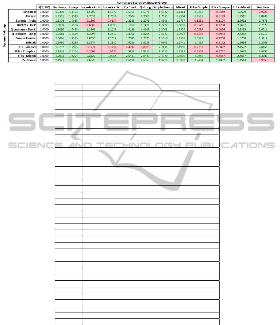
Table 1: Final rankings of teams or classes of closely related strategies w.r.t. metric U
1
.
Table 2: Final ranking of the individual strategies w.r.t. metric U
1
.
0.760787 Random [99, 100]
0.758874 Always 100
0.754229 Always 99
0.754138 Zeuthen Strategy - Positive
0.744326 Mixed - L(y-g) E(x-g) H(x-g), 80%); (100, 20%)
0.703589 Simple Trend - K = 3, Eps = 0.5
0.681784 Mixed - TFT (y-g), 80%); (R[99, 100], 20%)
0.666224 Simple Trend - K = 10, Eps = 0.5
0.639572 Simple Trend - K = 25, Eps = 0.5
0.637088 Mixed - L(x) E(x) H(y-g), 80%); (100, 20%)
0.534378 Mixed - L(y-g) E(x-g) H(x-g), 80%); (100, 10%); (2, 10%)
0.498134 Q Learn - alpha= 0.2, discount= 0.0
0.497121 Q Learn - alpha= 0.5, discount= 0.0
0.496878 Q Learn - alpha= 0.5, discount= 0.9
0.495956 Q Learn - alpha= 0.2, discount= 0.9
0.493640 Q Learn - alpha= 0.8, discount= 0.0
0.493639 Buckets - (Fullest, Highest)
0.493300 Q Learn - alpha= 0.8, discount= 0.9
0.492662 TFT - Low(y-g) Equal(x-g) High(x-g)
0.452596 Zeuthen Strategy - Negative
0.413992 Buckets - PD, Retention = 0.5
0.413249 Always 51
0.412834 Buckets - PD, Retention = 0.2
0.408751 Buckets - PD, Retention = 0.8
0.406273 Buckets - (Fullest, Random)
0.390303 TFT - Simple (y-g)
0.387105 Buckets - (Fullest, Newest)
0.334967 Buckets - (Fullest, Lowest)
0.329227 TFT - Simple (y-2g)
0.316201 Random [2, 100]
0.232063 Mixed - L(y-g) E(x-g) H(x-g), 80%); (2, 20%)
0.164531 Mixed - L(x) E(x) H(y-g), 80%); (100, 10%); (2, 10%)
0.136013 TFT - Low(x) Equal(x) High(y-g)
0.135321 TFT - Low(x) Equal(x-2g) High(y-g)
0.030905 TFT - Low(x-2g) Equal(x) High(y-g)
0.030182 TFT - Low(x-2g) Equal(x-2g) High(y-g)
0.026784 Mixed - L(x) E(x) H(y-g), 80%); (2, 20%)
0.024322 Always 2
ICAART 2012 - International Conference on Agents and Artificial Intelligence
82
