NONLINEAR FEATURE CONSTRUCTION WITH EVOLVED
NEURAL NETWORKS FOR CLASSIFICATION PROBLEMS
Tobias Berka and Helmut A. Mayer
Department of Computer Sciences, University of Salzburg, Jakob-Haringer-Strasse 2, Salzburg, Austria
Keywords:
Neural network, Genetic algorithm, Nonlinear dimensionality reduction, Nonlinear feature construction,
Classification.
Abstract:
Predicting the class membership of a set of patterns represented by points in a multi-dimensional space crit-
ically depends on their specific distribution. To improve the classification performance, pattern vectors may
be transformed. There is a range of linear methods for feature construction, but these are often limited in their
performance. Nonlinear methods are a more recent development in this field, but these pose difficult optimiza-
tion problems. Evolutionary approaches have been used to optimize both linear and nonlinear functions for
feature construction. For nonlinear feature construction, a particular problem is how to encode the function in
order to limit the huge search space while preserving enough flexibility to evolve effective solutions. In this
paper, we present a new method for generating a nonlinear function for feature construction using multi-layer
perceptrons whose weights are shaped by evolution. By pre-defining the architecture of the neural network
we can directly influence the computational capacity of the function and the number of features to be con-
structed. We evaluate the suggested neural feature construction on four commonly used data sets and report
an improvement in classification accuracy ranging from 4 to 13 percentage points over the performance on the
original pattern set.
1 INTRODUCTION
Finding representative features of entities to describe
them with a pattern vector is an important step in any
modern classification system. Part of this task is the
extraction and selection of useful measures from the
objects to be classified. A potential next step is fea-
ture construction, where the initial measures are arith-
metically combined to form artificial features, which
are more suitable for classification than the original,
domain-specific patterns.
Historically, feature construction is a modern ex-
tension of traditional statistical techniques such as
multi-dimensional scaling, principal component anal-
ysis, or factor analysis. Nowadays, these are referred
to, and used predominantly as, dimensionality reduc-
tion techniques. Linear methods such as the singu-
lar value decomposition (SVD) have been studied in
great detail, and today there is a sound theoretical un-
derpinning of optimal linear methods and detailed al-
gorithmic knowledge of their implementation. The
use of the SVD in data mining and machine learning
is so frequent that even a superficial survey is beyond
any research paper. But as with all linear techniques,
there are limits to their expressiveness that surface
quickly in a variety of applications. Consequently, it
is an obvious step to turn to nonlinear methods, al-
though this must also be understood as a departure
from the guaranteed optimality enjoyed using linear
techniques. One of the most popular means to intro-
duce nonlinearity is the kernel trick (Aizerman et al.,
1964), where a nonlinear function is applied to the
original pattern vectors. It is used to make a transi-
tion into a kernel space, in the hope that the problem
is more easily solved in the transformed domain. But
there is of course a catch: the choice of this kernel
function.
There are two main research directions in re-
sponse to this problem. The first approach is to
choose a default kernel function out of a limited set,
such as polynomials or radial basis functions. Ev-
ery new component in a vector in the kernel space is
the result of applying the kernel function to a pair of
components of the original vector. Unfortunately, an
exhaustive construction of new features involves all
pairs of components in the source vectors. The result
is a quadratic increase in dimensionality. For low-
dimensional problems, which suffer from poor sepa-
ration of data points, this can actually be an advan-
tage, and support vector machines explicitly exploit
35
Berka T. and Mayer H. (2012).
NONLINEAR FEATURE CONSTRUCTION WITH EVOLVED NEURAL NETWORKS FOR CLASSIFICATION PROBLEMS.
In Proceedings of the 1st International Conference on Pattern Recognition Applications and Methods, pages 35-44
DOI: 10.5220/0003754200350044
Copyright
c
 SciTePress

that fact (Vapnik, 1995). The dimensionality problem
can be mitigated to some extent by using feature se-
lection, where relevant features are identified from the
initially computed range of candidate features. In any
case the increase in dimensionality is the exact oppo-
site of the desirable dimensionality reduction.
The second approach is to attempt to construct a
kernel function specifically for the task at hand. In
order to obtain a nonlinear function that leads to a re-
duction in dimensionality, we decided to follow this
direction in our work. We are using an evolutionary
algorithm (EA) (B¨ack, 1996) to construct nonlinear
kernel functions implemented by a multi-layer per-
ceptron (MLP) (Bishop, 1995). Neural networks gen-
erated by EAs have been studied extensively for the
construction of classifiers, e.g., (Yao, 1999; Coelho
et al., 2001; Mayer and Schwaiger, 2002).
Our key contribution is the following: we are not
evolving a neural classifier, but a multi-layer percep-
tron that maps the original input patterns to a trans-
formed space of reduced dimensionality. This gives
us additional flexibility in the choice of the classifica-
tion system, which operates on the optimized trans-
formed space. In addition, we can also use the neural
transformation function for other applications, such
as similarity-based search and retrieval.
Formally, we have a set X = {x
1
, ..., x
n
}
of d-dimensional, real-valued pattern vectors,
(∀i ∈ {1...n})

x
i
∈ R
d

. We construct a transfor-
mation function f
T
: R
d
→ R
d
′
to perform feature
construction. The function f
T
is implemented by an
MLP with d input neurons and d
′
output neurons.
The weights of the connections and biases of the
individual neurons are encoded in a bit genome.
Starting with a randomly initialized population of
MLPs we compute a fitness score based on the
performance of the constructed features, select the
fitter individuals, and apply standard operators for
mutation and crossover during reproduction. This
process is repeated until a sufficiently good solution
has been found.
We have conducted an experimental evaluation on
four data sets. Using jackknifing with a K-nearest-
neighbor (K-NN) classifier, we have compared the
classification accuracy of the best solution against the
performance of the same classifier on the raw (un-
transformed) data set. The best solution is the fittest
MLP obtained in 50 independent runs over 2,000 gen-
erations with 50 individuals each. In our experiments,
we outperformed the base classification accuracy by
4, 5, 12, and 13 percentage points on the data sets
used for comparison. We also give a comparison with
related work, however, the literature on related ap-
proaches does not give all the details on performance
assessment. Therefore, all of these comparisons must
be taken with a grain of salt. Nonetheless, the results
indicate the potential of evolutionary neural feature
construction.
We describe our approach in detail in Section 2,
and discuss the related work in Section 3. Our empir-
ical evaluation is described in Section 4. Lastly, we
summarize our findings in Section 5.
2 OUR APPROACH
For the purpose of generating a nonlinear transforma-
tion function we evolvethe weights of fully connected
feed-forward networks with a single hidden layer. For
a data set with d features and a user-specified reduced
dimensionality of d
′
components, we have chosen a
network topology with d input neurons, d hidden neu-
rons and d
′
output neurons (or d − d − d
′
topology).
Hence the d-dimensional input pattern is transformed
to a d
′
-dimensional output pattern. An exemplary net-
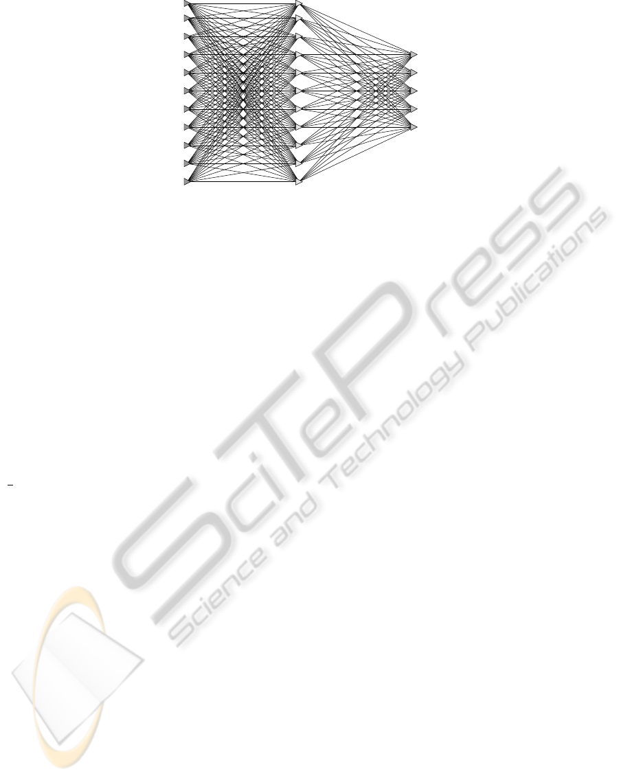
work is depicted in Figure 1. This topology has been
determined experimentally and performed well for all
of our benchmark experiments. We thus recommend
it as a starting point for other data sets as well.
The choice of a suitable d
′
is not easy. For our
evaluation, we have chosen d
′
according to experi-
ments reported in related literature. In general, we
recommend using an SVD to compute the singular
values of the data matrix and plotting them on a loga-
rithmic scale to reveal potential cut-off thresholds for
a rank reduction. This threshold should also serve as
a reasonable value for d
′
.
In our work, we are not using any learning al-
gorithms, such as error back-propagation or Hebbian
learning, to adapt the weights of the neural networks.
Instead, the optimization of the weights is the sole re-
sponsibility of the EA. This evolution of weights can
be viewedas evolutionary training of a network. Con-
ventionally, this strategy is used in scenarios where
training patterns are not or hardly available, such
as the evolution of robotic neurocontrollers (Ziemke
et al., 1999). However, own work also showed that
evolutionary training may even outperform conven-
tional training algorithms in problems with given in-
put/output patterns (Mayer and Mayer, 2006).
The activation function of all hidden neurons is
the standard sigmoid function, which is responsible
for the nonlinear mapping implemented by the neu-
ral network. The input and output neurons have lin-
ear activation functions (i.e., the identity function),
which is very common for input neurons. We based
our choice for the output neuron’s activation function
on the fact that certain classes of patterns may already
ICPRAM 2012 - International Conference on Pattern Recognition Applications and Methods
36


















x
1
x
2
x
3
x
4
x
5
x
6
x
7
x
8
x
9
x
10
x
11

















→ →





y
1
y
2
y
3
y
4
y
5





Figure 1: The structure of the network constructing five features out of eleven for the wine data set (see Table 1). The
network’s basic topology is used for all data sets: an initial input layer with d input neurons for the d features of the raw data
set, a hidden layer with d neurons, also, and an output layer with d
′
neurons for the d
′
constructed features. The single layers
of the networks are fully connected.
be arranged in distinct clusters of a certain distance,
which might be reduced because the sigmoid function
restricts output values to the unit interval.
The genotype of the network simply consists of
all the network’s weights and biases encoded in a
bit string. We restrict each weight to the interval
[−10, +10] using eight bits to encode a single weight
or bias. All neurons except the input neurons have
a bias value. For a network with 90 weights and 10
biases, the length of the chromosome is 800 bits.
The two genetic operators comply with the usual
choices without any specific adaptations. The stan-
dard bit-flip mutation is applied with a mutation rate
of
1
l
, where l is the chromosome length. This means
that only a single bit-flip operation is statistically ex-
pected in every generation for a single individual. The
crossover rate – the probability with which parents
exchange genetic information during reproduction –
was chosen to be p
c
= 0.6.
As a selection mechanism, we used binary tour-
nament selection. It operates by randomly choosing
two individuals, comparing their fitness score and dis-
carding the individual with the lower score. It thus
implements the survival of the fittest. The constant
population size is 50, and the number of generations
is set to 2,000 for all experiments. Overall, these set-
tings constitute a basic evolutionary algorithm with-
out problem-specific algorithmic adjustments.
The evaluation of the fitness of the individual neu-
ral networks adheres to a technique commonly used
in determining the quality of a feature subset. For
the latter there are two basic approaches, namely, the
filter and the wrapper approach (John et al., 1994).
With the filter approach a statistical measure is used
to assess the quality of a feature subset, while the
wrapper approach employs the accuracy of a classi-
fier. As usual, both approaches have their advantages
and drawbacks.
Essentially, the filter approach would allow fast
computation of the fitness, however, there is no gen-
eral guideline, which measures should be used to
achieve good classification performance for a spe-
cific classifier. In preliminary experiments, we used
the standard Fisher criterion (also used in (Guo and
Nandi, 2006)) in a filter approach resulting in im-
provements in classification performance after neu-
ral feature construction. The wrapper approach uses
the direct information on a classifier’s accuracy, hence
the performance is optimized, however at the price of
computational cost and classifier specificity. Using a
K-NN classifier, the wrapper method produced better
results with acceptable computational cost. These are
the results we present in this paper.
A problem with our approach stems from the fact
that the number of connections increases with the
square of the number of neurons. We are using a
neural network topology with one hidden layer and
allow connections only between neurons in adjacent
layers. For i input neurons, h hidden neurons and o
output neurons, we have a total connection count C of
C = ih+ho. In our experiments, the number of hidden
neurons was equal to the number of hidden neurons,
meaning that C = i
2
+ io. Assuming that we always
perform a dimensionality reduction, we have o < i,
and therefore O(C) = O(i
2
+ io) ≤ O(2i
2
) = O(i
2
).
Since we have to encode a weight for every con-
nection, the length of the bit string may exceed fea-
sible values as the number of connections increases.
This poses a problem, as the number of input neu-
rons is dictated by the number of features in a given
data set. Consequently, we believe that the specific
approach presented here is currently only applicable
to data sets with a moderate number of features. How-
ever, it should be noted that the best results in this pa-
NONLINEAR FEATURE CONSTRUCTION WITH EVOLVED NEURAL NETWORKS FOR CLASSIFICATION
PROBLEMS
37

per have been achieved with the largest network en-
coded with a hefty 11,752 bits (c.f. the ionosphere re-
sults in Table 3).
3 RELATED WORK
Spectral, singular value or eigenvalue techniques are
perhaps the most common family of methods for fea-
ture space transformations. These are the classic
foundation of linear projection methods for dimen-
sionality reduction by projection onto the principal
axes. Related to the evolutionary aspects of our ap-
proach, (Aggarwal, 2010) introduces an evolutionary
technique to construct a linear dimensionality reduc-
tion of the feature vector. In short, the evolution gen-
erates a low-dimensional hyperplane, on which the
original data are projected. These projected points are
then presented to a classifier for computing the fitness
and evaluating the overall quality. The dimensionality
of the reduced space can be adjusted by the user, but
the algorithm may occasionally go lower than that.
In digital image processing, the principal com-
ponent analysis (PCA) traditionally used for dimen-
sionality reduction has been combined with the ker-
nel trick to form the nonlinear component analy-
sis (Sch¨olkopf et al., 1998), which corresponds to
solving an eigenvalue problem in the kernel space. It
can be used to construct nonlinear features for feature
extraction (Chin and Suter, 2006) or various image
enhancement tasks (Kim et al., 2005).
More closely related to our approach, (Guo and
Nandi, 2006) introduce the use of genetic program-
ming for nonlinear feature construction. Here, fea-
tures are constructed by evolved programs using a
pre-defined set of arithmetic operators and the raw
features as program input. An even earlier attempt
to nonlinear feature construction is based on the
construction of nonlinear decision trees (Ittner and
Schlosser, 1996) using polynomial functions to re-
strict the search space.
4 EMPIRICAL EVALUATION
Our choice of data sets is based on related work so as
to compare the performance of different approaches.
The four data sets have been obtained from the UCI
Machine Learning Repository (Frank and Asuncion,
2010) whose kind support we wish to acknowledge.
Table 1 describes the data sets used in the following
experiments.
To compare the performance of our approach with
the feature construction by genetic programming de-
tailed in (Guo and Nandi, 2006), we are using the
Breast Cancer Wisconsin (Diagnostic) data set (Street
et al., 1993), which contains image features extracted
from fine needle aspirates of breast mass for the
discrimination of benign and malignant tissue. It
contains 569 patterns with 32 features, which are
uniquely labeled to belong to one of 2 classes.
We have selected two data sets for comparison
with the evolution of representative patterns for lin-
ear dimensionality reduction (Aggarwal, 2010). The
Ionosphere data set (Sigillito et al., 1989) contains
radar return signals. Here, we are instructed to dis-
criminate between “good” and “bad” radar return sig-
nals. Good return signals may be used to reveal
some structures in the ionosphere, whereas bad sig-
nals merely pass through it. This data set contains 251
instances with 34 features. In addition, we are also
using the Image Segmentation data set (Scott et al.,
1998), which consists of 2,310 patterns with 19 fea-
tures. It is based on an image processing task and
contains instances of 7 real-world image region cate-
gories for machine vision (brickface, cement, foliage,
grass, path, sky and window).
A data set that traditionally requires some pre-
processing contains chemical data of wine sam-
ples (Cortez et al., 2009), which are categorized into
six quality classes, because the individual features
come from disparate scales of measurement. We have
selected this data set because we can demonstrate the
computational ability of our approach on the raw, un-
processed data. The red wine sub-collection, with
1599 patterns and 11 features, completes the data sets
used in the experiments.
For all of these data sets we consulted the related
work to determine a suitable reduced dimension of the
transformed space. The reduced dimensionalities and
the neural network topology used in our experimental
evaluations are given in Table 2.
We experimentally determined some evolution pa-
rameters by conducting trial runs on the data sets, and
consistently used the following setting:
1. We found a population size of 50 individuals to
be sufficient for all four data sets. Attempts to
increase the population size did not lead to any
improvements, whereas lowering it decreased the
performance of the optimization.
2. In these experiments the best solution was typ-
ically found after approximately 1,500 genera-
tions. To be safe we set the number of generations
to 2,000.
3. We execute all experiments in 50 independent
runs. The optimal result reported is always the
ICPRAM 2012 - International Conference on Pattern Recognition Applications and Methods
38

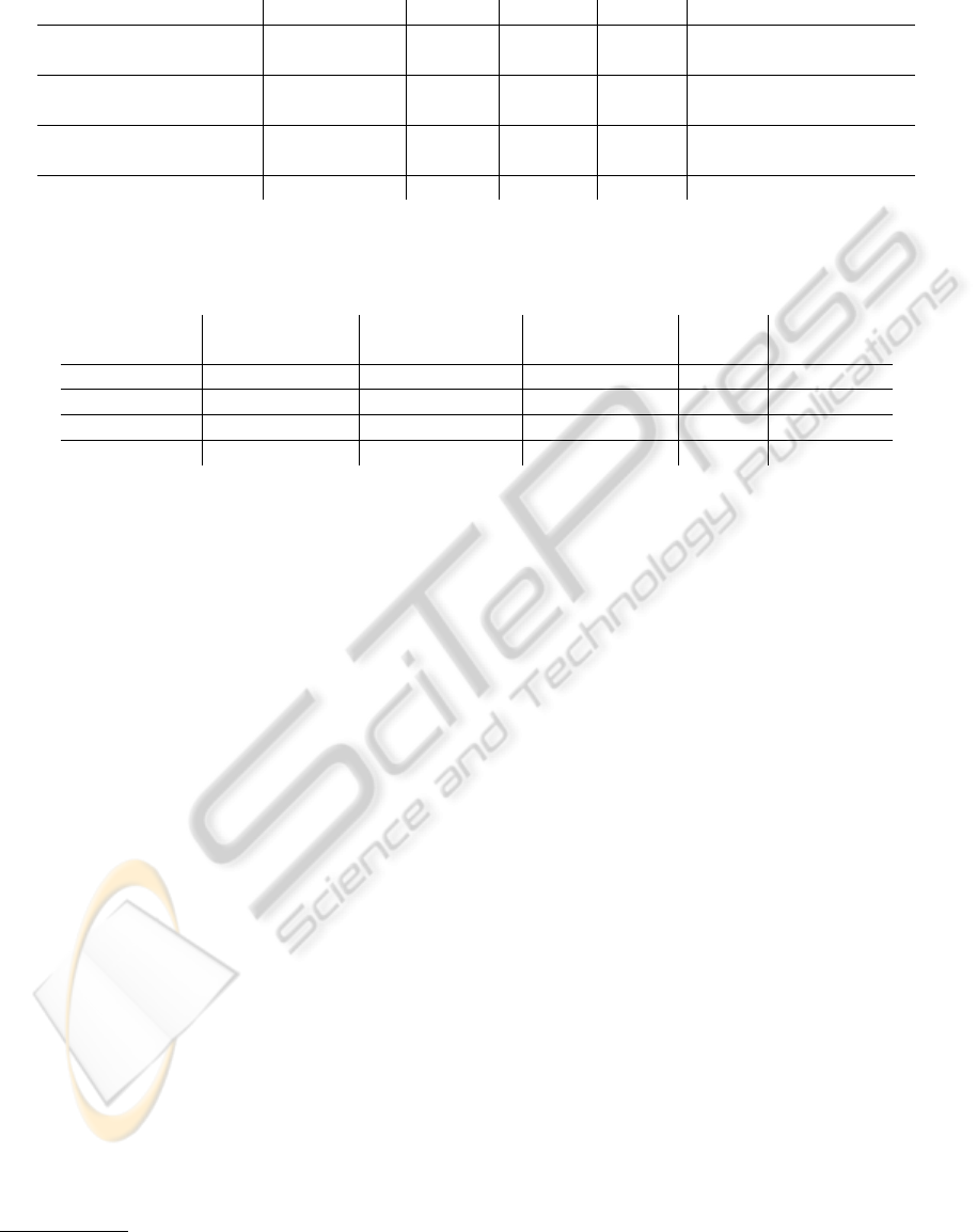
Table 1: Overview of the data sets used for evaluation. As indicated in Section 2, the presented approach may not be amenable
to data sets with a large number of features, hence the data sets have been chosen accordingly.
Full Name Short Name Patterns Features Classes Reference
Breast Cancer Cancer 569 32 2 (Guo and Nandi, 2006),
Wisconsin (Diagnostic) (Street et al., 1993)
Image Segmentation Segmentation 2310 19 7 (Aggarwal, 2010),
(Scott et al., 1998)
Ionosphere Ionosphere 251 34 2 (Aggarwal, 2010),
(Sigillito et al., 1989)
Red Wine Wine 1599 11 6 (Cortez et al., 2009)
Table 2: Template neural networks used for evolutionary feature construction. A neural network topology x−y− z refers to
a neural network with x input neurons, a single hidden layer with y hidden neurons, and z output neurons. The number of
dimensions in the reduced space is based on the related literature.
Data Set Original Neural Network Reduced Neuron Connection
Dimensionality Topology Dimensionality Count Count
Cancer 30 30− 30− 3 3 63 990
Segmentation 19 19 − 19 − 4 4 42 437
Ionosphere 34 34− 34− 7 7 75 1394
Wine 11 11− 11− 5 5 27 176
single best solution found for a given data set in
all of these runs.
The complete Java software implementing the
evolution of neural networks and the K-NN classifier
has been developed at our institution, and is mainly
based on the JEvolution package, written by one of
the authors, and the neural network package Boone
1
.
A single run as specified above required approxi-
mately 30 minutes on a CPU of the Intel Nehalem
architecture family.
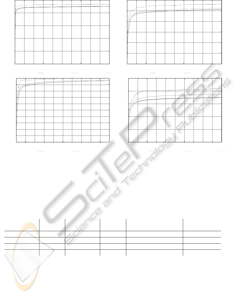
To visualize the evolutionary success Figure 2 de-
picts the development of the fitness scores over the
number of generations. These plots contain three
measures to convey a more detailed picture of the
development of the populations across all runs. The
mean average fitness is the average of the fitness score
over all runs and individuals within the same genera-
tion. The mean best fitness is the average of the high-
est fitness score achieved in each run in each genera-
tion. The best fitness score is the highest fitness score
found for any individual in all runs per generation.
Above measurements reveal that most of the evo-
lutionary progressis achievedwithin the first 200 gen-
erations. Apparently, the problem of constructing a
suitable transformation function has sufficiently many
sound solutions, so that the genetic algorithm can
make immediate and substantial improvements. The
rather sharp transition to a small rate of progress is
typical for artificial evolution, but improvements may
1
All the credits for Boone go to our colleague August
Mayer.
be found along the entire interval of measurement.
Another effect that is well visible in these dia-
grams is the rather large discrepancy between the av-
eraged fitness scores and the fitness of the best so-
lution. Preliminary investigations indicate that the
initial average fitness of a population determines the
maximum fitness which can be found throughout the
entire evolution. This suggest that it may be advisable
to perform an initial step of high-throughput screen-
ing. In this approach, we initially construct a ran-
domly generated population that is one or two orders
of magnitude larger than the population size of the
evolutionary algorithm.
In any case, the ultimate measure of success is the
classification accuracy in the transformed space com-
pared to that on the original data, and in relation to
the performance reported in related work. It should
be noted that comparisons to related work are more
of a qualitative manner, as not all necessary details
are given, e.g., in (Aggarwal, 2010) random subsets
of the original data sets are used for evolution of the
linear hyperplanes.
In order to provide a solid baseline for the perfor-
mance of neural feature construction we have used the
following setup:
1. The results of jackknife (or leave-one-out) eval-
uation using a K nearest-neighbor classifier with
K = 1, ..., 30 on the original data set act as a per-
formance baseline.
2. During evolution jackknifing evaluation is per-
formed on the transformed feature vectors of the
NONLINEAR FEATURE CONSTRUCTION WITH EVOLVED NEURAL NETWORKS FOR CLASSIFICATION
PROBLEMS
39

0.5
0.6
0.7
0.8
0.9
1
0 200 400 600 800 1000 1200 1400 1600 1800 2000
fitness
generation
mean average fitness mean best fitness best fitness
0.4
0.5
0.6
0.7
0.8
0.9
1
0 200 400 600 800 1000 1200 1400 1600 1800 2000
fitness
generation
mean average fitness mean best fitness best fitness
0.8
0.82
0.84
0.86
0.88
0.9
0.92
0.94
0.96
0.98
1
0 200 400 600 800 1000 1200 1400 1600 1800 2000
fitness
generation
mean average fitness mean best fitness best fitness
0.5
0.55
0.6
0.65
0.7
0.75
0 200 400 600 800 1000 1200 1400 1600 1800 2000
fitness
generation
mean average fitness mean best fitness best fitness
Figure 2: Illustration of the fitness scores of 50 independent experimental runs with 50 individuals over 2,000 generations
using the breast cancer data set (top left), the segmentation data set (top right), the ionosphere data set (bottom left) and the
red wine data set (bottom right). The network topologies are those given in Table 2. The fitness function is the classification
accuracy of a K-nearest-neighbor classifier with K = 1. The mean average fitness is the mean of the average fitness per
generation of all runs. The mean best fitness is the mean fitness over all runs of the best individual in a specific generation.
The best fitness is the fitness score of the single best individual from all runs per generation.
Table 3: Comparison of the classification accuracy obtained by neural feature construction with the results reported in related
work. Comparisons to related work should be viewed as qualitative trends, as performance measurement could not be re-
produced in full detail. All percentages have been rounded for clarity. Improvement scores are computed from the rounded
figures and are given in percentage points (pp).
Data Set Baseline Accuracy in Our Best Improvement over Features
Short Name Accuracy Related Work Accuracy Baseline / Related Work Raw / Reduced
Cancer 93% 99% 97% 4 pp / -2 pp 30 / 3
Segmentation 84% 78% 96% 12 pp / 18 pp 19 / 4
Ionosphere 87% 92% 100% 13 pp / 8 pp 34 / 7
Wine 62% 62% 67% 5 pp / 5 pp 11 / 5
full data set to determine the fitness of the individ-
ual MLPs. For fitness evaluation we chose K = 1,
as this setting produced the highest classification
accuracy in all four data sets.
3. We used the best individual across all runs as
transformation function and re-evaluated the jack-
knifing K-NN classifier performance of the full,
transformed data set in the range of K = 1, ..., 30.
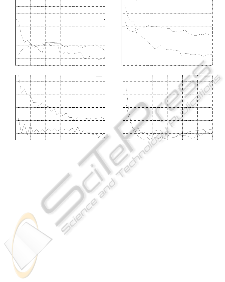
The jackknifing (or leave-one-out) classification
accuracy performance evaluation on the raw data and
the transformed data generated by the best MLP are
plotted in Figure 3. For comparability with related
approaches, we have taken the following performance
figures from the related work:
• Cancer: 99% in (Guo and Nandi, 2006),
• Segmentation: 78% in (Aggarwal, 2010),
• Ionosphere: 92% in (Aggarwal, 2010),
• Wine: 62% in (Cortez et al., 2009) with T = 0.5.
Since our fitness evaluation employed a K-NN
ICPRAM 2012 - International Conference on Pattern Recognition Applications and Methods
40

0.9
0.91
0.92
0.93
0.94
0.95
0.96
0.97
0.98
0.99
1
0 5 10 15 20 25 30
classification accuracy
K
raw data
best MLP
0.5
0.6
0.7
0.8
0.9
1
0 5 10 15 20 25 30
classification accuracy
K
raw data
best MLP
0.8
0.82
0.84
0.86
0.88
0.9
0.92
0.94
0.96
0.98
1
0 5 10 15 20 25 30
classification accuracy
K
raw data
best MLP
0.5
0.52
0.54
0.56
0.58
0.6
0.62
0.64
0.66
0.68
0.7
0 5 10 15 20 25 30
classification accuracy
K
raw data
best MLP
Figure 3: Illustration of the jackknifing performance evaluation of a K-nearest-neighbor classifier on the original data and the
transformed data (by the best MLP) over K for breast cancer (top left), segmentation (top right), ionosphere (bottom left) and
red wine (bottom right).
classifier with K = 1, it is not surprising that the best
results are obtained with this setting. For increasing
values of K we see a drop in classification accuracy
on the transformed data. This may indicate that the
evolved neural transformation manages to improve
the local neighborhood of individual points, but does
not succeed in creating clusters of data points for spe-
cific categories. However, we notice a clear improve-
ment of the classification accuracy over the baseline
for low values of K. In this range the best perfor-
mance of the K-NN classifier on three out of four of
the original, unprocessed data sets (except the cancer
data set) can be found.
We conducted several experiments using larger
values of K in the fitness function. The evolution suc-
ceeded in optimizing these populations, but the solu-
tions produced with K = 1 performed best.
A summary of the best results obtained in all ex-
perimental runs, the performance baseline on the raw
data set and a comparison with the values reported in
the related literature is given in Table 3.
What stands out in this performance comparison is
the fact that our approach provides only limited gains
on data sets that are either “easy” such as the cancer
data set, or sets that are “hard” such as the wine data
set. The highest improvements were achieved on data
sets, which have a baseline classification accuracy be-
tween these two, namely, the segmentation and iono-
sphere data sets. This may be based on the following
reasons:
• With “easy” data sets it is difficult to achieve im-
provements, because only few patterns are mis-
classified anyway. Consequently, it is difficult to
modify a neural network to improve on these few
patterns, while at the same time preserving correct
classification of all others.
• With “hard” data sets our approach is being ham-
pered by the continuous nature of the neural net-
works. If there is a high degree of confusion in
the local neighborhood of a pattern, containing a
mix of patterns from other categories, it is difficult
for a neural network to improve separation, as the
standard activation function we used in this work
is continuous and monotonous. Consequently, ad-
jacent patterns in the original input space will not
be far apart in the evolved transformed space.
• Data sets with an intermediate level of difficulty
provide plenty of room for improvement. Conse-
NONLINEAR FEATURE CONSTRUCTION WITH EVOLVED NEURAL NETWORKS FOR CLASSIFICATION
PROBLEMS
41

0
200
400
600
800
1000
1200
1400
-2000 -1500 -1000 -500 0
benign malignant
-5
0
5
10
15
-55 -50 -45 -40 -35 -30 -25 -20 -15 -10
benign malignant
-50
0
50
100
150
-300 -250 -200 -150 -100 -50
BRICKFACE
SKY
FOLIAGE
CEMENT
WINDOW
PATH
GRASS
-10
0
10
20
30
40
50
-30 -20 -10 0 10 20
BRICKFACE
SKY
FOLIAGE
CEMENT
WINDOW
PATH
GRASS
-1
-0.5
0
0.5
1
1.5
2
2.5
3
3.5
-4 -3 -2 -1 0 1
good bad
-60
-50
-40
-30
-20
-10
0
10
-40 -30 -20 -10 0 10 20 30 40
good bad
0
20
40
60
80
100
0 20 40 60 80 100
3 4 5 6 7 8
-25
-20
-15
-10
-5
0
-8 -6 -4 -2 0 2 4 6 8 10
3 4 5 6 7 8
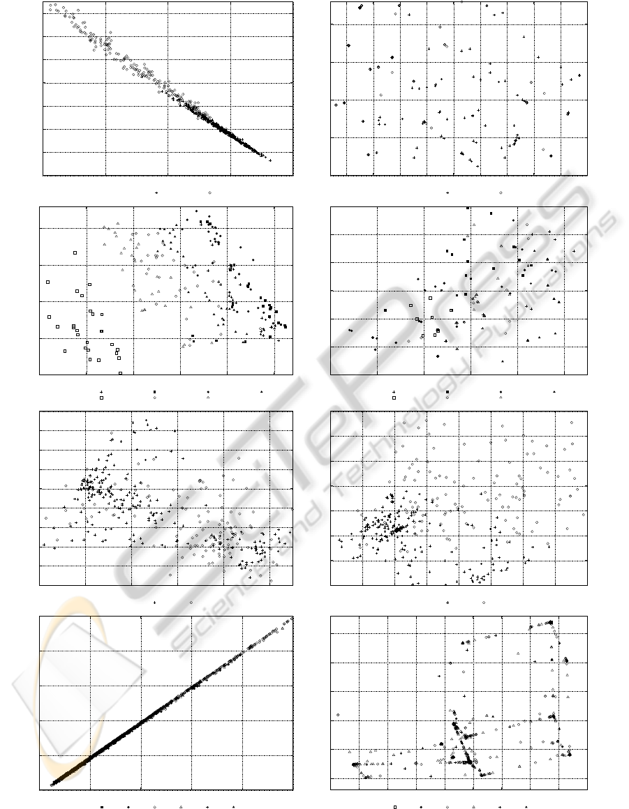
Figure 4: All data points in the cancer (top), segmentation (middle high), ionosphere (middle low) and wine wine data set
(bottom) projected onto the first two principal axes of the original data (left) and the transformed data generated by the best
MLP (right). Some outliers have been omitted for clarity.
ICPRAM 2012 - International Conference on Pattern Recognition Applications and Methods
42

quently, decent improvement within the available
headroom is possible.
In order to provide further insights into the ef-
fect of neural feature transformation, a graphical rep-
resentation of the patterns in the original and trans-
formed feature space is given. Since the data are of
high dimensionality, we employed principal compo-
nent analysis for a two-dimensional projection of pat-
terns, which can conveniently be plotted in a diagram.
Here, we can see all patterns projected onto the plane
defined by the two orthogonal directions with max-
imal variance in the data set. These directions are
not necessarily the best directions in terms of sepa-
ration of the categories, but are based on the variance
within the entire set of patterns. We show the two-
dimensional principal component plots of the original
and mapped points in Figure 4.
These plots can give us a fairly good understand-
ing of the classification accuracy with varying K as
depicted in Figure 3. Despite the fact that they are
only two-dimensional and there are one or more di-
mensions missing, they do illustrate the ability of
the evolved neural transformation functions to break
up linear dependencies within the first two principal
axes. We can clearly see the ability to optimize the
local neighborhood of most data points in terms of
class membership. But we can also see their inability
to create distinct clusters for specific categories.
5 SUMMARY AND
CONCLUSIONS
In this paper we have introduced the use of multi-
layer perceptrons as nonlinear functions for feature
construction in classification tasks. Our key contri-
bution is that we evolve a transformation function in-
stead of a classifier. An evolutionary algorithm is used
to evolve weights and biases of the neural networks
directly encoded in a bit string. The classification ac-
curacy of a K-nearest-neighbor classifier with K = 1
has been used to determine the fitness of the neural
networks transforming the original feature vectors to
a lower dimension. Plots of the development of the
fitness values over time indicate that this approach is
able to find excellent solutions, and that a stable opti-
mization does take place. We evaluated this approach
on four commonly used data sets using jackknifing
(leave-one-out) for evaluating the classification accu-
racy. To the extent possible we compared the perfor-
mance of our approach with related work. In addi-
tion we measured a performance baseline on the raw
(untransformed) data. The neural feature construction
presented in this paper delivers performance improve-
ments of 4, 5, 12, and 13 percentage points over these
baseline figures, outperforming the related work in
three out of four cases. We believe that we have thus
delivered a proof of concept for evolutionary neural
transformation functions on actual data.
REFERENCES
Aggarwal, C. (2010). The Generalized Dimensionality Re-
duction Problem. In Proceedings of the SIAM Interna-
tional Conference on Data Mining, SDM 2010, pages
607–618. SIAM.
Aizerman, A., Braverman, E. M., and Rozoner, L. I. (1964).
Theoretical Foundations of the Potential Function
Method in Pattern Recognition Learning. Automation
and Remote Control, 25:821–837.
B¨ack, T. (1996). Evolutionary Algorithms in Theory and
Practice. Oxford University Press.
Bishop, C. M. (1995). Neural Networks for Pattern Recog-
nition. Oxford University Press, Inc., New York, NY,
USA.
Chin, T.-J. and Suter, D. (2006). Incremental Kernel PCA
for Efficient Non-linear Feature Extraction. In Pro-
ceedings of the 17th British Machine Vision Confer-
ence, pages 939–948. British Machine Vision Associ-
ation.
Coelho, A., Weingaertner, D., and von Zuben, F. J. (2001).
Evolving Heteregeneous Neural Networks for Classi-
fication Problems. In Proceedings of the Genetic and
Evolutionary Computation Conference, pages 266–
273, San Francisco. Morgan Kaufmann.
Cortez, P., Cerdeira, A., Almeida, F., Matos, T., and Reis, J.
(2009). Modeling Wine Preferences by Data Mining
from Physicochemical Properties. Decision Support
Systems, 47(4):547–553.
Frank, A. and Asuncion, A. (2010). UCI Machine Learning
Repository.
Guo, H. and Nandi, A. K. (2006). Breast Cancer Diagnosis
using Genetic Programming Generated Feature. Pat-
tern Recognition, 39(5):980–987.
Ittner, A. and Schlosser, M. (1996). Discovery of Rele-
vant New Features by Generating Non-Linear Deci-
sion Trees. In Proceedings of the Second International
Conference on Knowledge Discovery and Data Minin,
pages 108–113. AAAI.
John, G. H., Kohavi, R., and Pfleger, K. (1994). Irrelevant
Features and the Subset Selection Problem. In In-
ternational Conference on Machine Learning, pages
121–129.
Kim, K. I., Franz, M. O., and Scholkopf, B. (2005). Itera-
tive Kernel Principal Component Analysis for Image
Modeling. IEEE Transactions on Pattern Analysis and
Machine Intelligence, 27(9):1351–1366.
Mayer, A. and Mayer, H. A. (2006). Multi–Chromosomal
Representations in Neuroevolution. In Proceedings
of the Second IASTED International Conference on
Computational Intelligence. ACTA Press.
NONLINEAR FEATURE CONSTRUCTION WITH EVOLVED NEURAL NETWORKS FOR CLASSIFICATION
PROBLEMS
43

Mayer, H. A. and Schwaiger, R. (2002). Differentiation of
Neuron Types by Evolving Activation Function Tem-
plates for Artificial Neural Networks. In Proceedings
of the 2002 World Congress on Computational Intelli-
gence, International Joint Conference on Neural Net-
works, pages 1773–1778. IEEE.
Sch¨olkopf, B., Smola, A., and M¨uller, K.-R. (1998). Non-
linear Component Analysis as a Kernel Eigenvalue
Problem. Neural Computation, 10(5):1299–1319.
Scott, M. J. J., Niranjan, M., and Prager, R. W. (1998).
Realisable Classifiers: Improving Operating Perfor-
mance on Variable Cost Problems. In Proceedings of
the British Machine Vision Conference 1998. British
Machine Vision Association.
Sigillito, V. G., Wing, S. P., Hutton, L. V., and Baker, K. B.
(1989). Classification of Radar Returns from the Iono-
sphere using Neural Networks. Johns Hopkins APL
Tech. Dig, 10:262–266.
Street, W. N., Wolberg, W. H., and Mangasarian, O. L.
(1993). Nuclear Feature Extraction for Breast Tumor
Diagnosis. In IS&T/SPIE 1993 International Sym-
posium on Electronic Imaging: Science and Technol-
ogy, volume 1905 of Society of Photo-Optical Instru-
mentation Engineers (SPIE) Conference Series, pages
861–870.
Vapnik, V. N. (1995). The Nature of Statistical Learning
Theory. Springer-Verlag New York, Inc., New York,
NY, USA.
Yao, X. (1999). Evolving Artificial Neural Networks. Pro-
ceedings of the IEEE, 87(9):1423–1447.
Ziemke, T., Carlsson, J., and Bod´en, M. (1999).
An Experimental Comparison of Weight Evolution
in Neural Control Architectures for a ’Garbage-
Collecting’ Khepera Robot. In Proceedings of
the 1st International Khepera Workshop. HNI–
Verlagsschriftenreihe.
ICPRAM 2012 - International Conference on Pattern Recognition Applications and Methods
44