SOLVING THE 3D CONTAINER SHIP LOADING

PLANNING PROBLEM BY REPRESENTATION

BY RULES AND BEAM SEARCH

Anibal Tavares de Azevedo

, Cassilda Maria Ribeiro

, Galeno José de Sena

Antônio Augusto Chaves

, Luis Leduíno Salles Neto

and Antônio Carlos Moretti

Mathematics Department, State of São Paulo University, Av. Dr. Ariberto Pereira da Cunha, 333, Guaratinguetá, Brazil

Department of Science and Technology, Federal University of São Paulo, São José dos Campos, Brazil

Mathematics Department, State University of Campinas, Rua Sérgio Buarquede Holanda, 651, Campinas, Brazil

Keywords: 3D Container ship Stowage, Combinatorial Optimization, Beam Search Method.

Abstract: This paper formulates the 3D Container ship Loading Planning Problem (3D CLPP) and also proposes a

new and compact representation to efficiently solve it. Containers on board a Container ship are placed in

vertical stacks, located in different sections. The only way to access the containers is through the top of the

stack. In order to unload a container at a given port j, it is necessary to remove the container whose

destination is the port j+1, because it is located above the container we want to download. This operation is

called “shifting”. A ship container carrying cargo to several ports may require a large number of shifting

operations. These operations spend a lot of time and cost and can be avoided by using efficient stowage

planning. The key objective of the stowage planning is to minimize the number of container movements and

also the ship instability. The binary formulation of this problem is properly described and also an alternative

formulation called representation by rules is proposed. A Beam Search is combined with representation by

rules to solve the 3D CLPP in manner that ensures that every solution analyzed in the optimization process

is compact and feasible.

1 INTRODUCTION

The operational efficiency of a port depends on a

proper container moving planning, called as

“stowage planning”, especially because the

Container ship loading process demands unloading

service time, and this has a cost. According to

Dubrovsky et al. (2002), the charge of the ship for

moving containers could be high, costing about $200

per container move. Thus, the objective of the

stowage planning for the Container ship is to

minimize the number of unnecessary movements. It

is also important to point out that other criteria must

be observed such as Container ship stability (weight

of the containers), type of containers (standard,

hazardous, etc), and others (Ambrosino et al., 2006;

Avriel et al., 1998; Wilson and Roach, 2000). In this

Paper, the problem that will be solved is the one that

shows how to create a proper container moving

planning, which minimizes the unnecessary

container movements and also the instability. The

development of an efficient method could be derived

observing the cellular structure of the Container

ship, as showed by Figure 1, which forces the

containers to be organized in vertical stacks. As a

consequence the containers located on the top of the

stack have be moved in order to allow the unloading

of the containers located at the bottom of the stack.

This rearrangement is called as a necessary shift, and

it occurs because the containers can be removed

from the Container ship through the top of the stack.

Figure 1: The Container ship cellular structure from

Wilson and Roach (2000).

As showed by (Avriel et al., 1998), the 2D

Container ship loading planning problem (CLPP)

132

Tavares de Azevedo A., Maria Ribeiro C., José de Sena G., Augusto Chaves A., Leduíno Salles Neto L. and Carlos Moretti A..

SOLVING THE 3D CONTAINER SHIP LOADING PLANNING PROBLEM BY REPRESENTATION BY RULES AND BEAM SEARCH.

DOI: 10.5220/0003757801320141

In Proceedings of the 1st International Conference on Operations Research and Enterprise Systems (ICORES-2012), pages 132-141

ISBN: 978-989-8425-97-3

 2012 SCITEPRESS (Science and Technology Publications, Lda.)

could be formulated as a 0-1 binary linear model,

whose optimal solution can be found by assuming

that the number of containers to be shipped, along

with their origin and the destination ports, are known

in advance. However, this binary model is limited

for small instances, since the number of binary

variables and constraints substantially grows with

the number of ports and Container ship dimensions.

This binary model also does not take into account

the consistency of the container’s allocation as the

ship proceeds from port to port.

It was also proved by (Avriel et al., 2000) that

the 2D CLPP is NP-Complete and this motivates the

development of a series of heuristics and meta-

heuristics to obtain good solutions for this problem.

(Avriel et al., 1998) proposed the Suspensory

Heuristic Procedure, which avoids the binary model

problem by observing only the Container ship

arrangement and the containers that must be loaded

for each specific port. The Paper also described how

to generate instances for the CLPP. Dubrovsky et al.

developed a Genetic Algorithm with a compact

solution encoding, which consists of a string with

sections equal to the number of ports, and each

section is composed by four vectors related to the

number of necessary shifts (Dubrovsky et al., 2002).

(Ambrosino 2006, 2010) also introduced and tested

in the model the notion of stability by considering

that each container has a weight.

Due to the CLPP being a complex problem, this

Paper proposes a two-stage procedure. The Beam

search manipulates the encoded solutions, which are

then evaluated by a decoding algorithm that consists

of the loading and the unloading Container ship

simulation for every/each port. This decoding

procedure is performed in a manner that the size of

the search space can be reduced and human

knowledge may be properly incorporated. This

encoding was called as the representation by rules.

Section 2 presents the CLPP mathematical model.

Section 3 explains the encoding, used by Beam

Search Method, and its advantages. Section 4 details

the Beam Search Method implementation. Section 5

presents and discusses the computational results and

Section 6 presents the conclusions and future works.

2 MATHEMATICAL MODEL

A Container ship has its capacity measured in terms

of TEU (Twenty-foot Equivalent Units). For

example, a ship with 8000 TEUs is able to carry at

least 8000 twenty feet deep containers. The

Container ship has a cellular structure (see Figure 1)

where the containers are stored. These cells are

grouped in Sections, or Bays, where the containers

are stacked in forming vertical stacks. Then, a bay is

a group of cells where a certain number of

containers are organized, forming a series of vertical

stacks. Generally, each bay can lead to containers of

forty or twenty feet deep. Then, the bay could be

organized in horizontal lines numerated with r = 1,

2,…, R, in a way that line one represents the bottom

of the ship and line R is on the top of the ship, and

columns numerated with c = 1, 2, …, C, where

column 1 is the leftmost one.

For the sake of simplicity, without loss of

generality, it will be considered that:

(a) The Container ship will have a rectangular

format and can be represented by a matrix with

horizontal lines (r = 1, 2,…, R), vertical columns (c

= 1, 2, …, C) and bays (d = 1, 2,…, D) with

maximum capacity of R x C x D containers.

(b) The containers are all the same size and

weight.

arrives empty.

(d) The ship visits ports 2, 3,…, N and the

Container ship will be empty in the last port,

because the ship performs a circular route where

port N in fact represents port 1.

(e) In each port i = 1, 2,…, N the Container

ship can be loaded with containers whose destination

are ports i+1, …, N.

(f) The Container ship could always carry all

the containers available in each port and this will

never exceed the maximum Container ship capacity.

In addition to conditions (a)-(f), the number of

containers that must be loaded at a certain port is

given by a transportation matrix T of dimension (N-

(N-1), whose element T

represents the number

of containers from port i that must be transported to

the destination port j. This matrix is superior and

triangular, since T

=0 for every i

≥

The mathematical model in terms of linear

programming with binary variables for the 3D CLPP

is given by (1)-(6).

Min

)()1()()(

yxxf

αφ

−

;,,1,1,,1 NijNi LL +

−

(1)

S.a:

∑∑∑ ∑∑∑∑∑

+===

−

=== ==

=−

kji

ijv

Tdcrxdcrx

11 1

111 11

),,(),,(

;,,1,1,,1 NijNi LL +

−

(2)

SOLVING THE 3D CONTAINER SHIP LOADING PLANNING PROBLEM BY REPRESENTATION BY RULES AND

BEAM SEARCH

133

∑∑∑

=+=+=

kjv

dcrydcrx

111

),,(),,(

;,,1,1,,1 RrNi LL =−=

;,,1 Cc L=

Dd ,,1 L=

(3)

0),,1(),,( ≥

− dcrydcry

;,,1,1,,1 RrNi LL =−=

;,,1 Cc L= Dd ,,1 L

(4)

∑∑ ∑ ∑ ∑

−

=+=+=

≤++

111

1),,1(),,(

ipvipj

dcrxdcrx

;1,,1,,,2 −== RrNi LL

;,,1 Cc L= Dd ,,1 L

(5)

1or 0),,( =dcrx

ijv

; 1or 0),,( =dcry

(6)

where: the binary variable

),,( dcrx

ijv

is defined as

if, in port i, the compartment (r,c,d) has a container

whose destination is port j and this container was

moved in port v, then the variable assumes value 1;

otherwise value 0 is assumed. The term

compartment (r,c,d) represents line r, column c for

the Container ship bay d. Similarly, variable

),,( dcry

is defined as if, in port i, the

compartment (r,c,d) has a container; then the

variable assumes value 1; otherwise value 0 is

assumed.

The objective function (1) it composed by two

terms that gives the total cost of moving a container

and the sum of instability measure for the Container

ship configuration in each port. It was assumed that,

for all ports, the container moving has the same and

unitary value. The constraint (2) is related to the

container conservation flow. In other words, the total

number of containers in the ship in a port i must be

equal to the number of containers that had been

loaded in all ports p = 1 2, ,…, i minus the total

number of containers unloaded in all ports p = 1, 2,

…, i. The constraint (3) obliges that each

compartment (r,c,d) of the Container ship in all ports

is occupied by at most one container. The constraint

(4) is related to the physical storage of the containers

in the ship, and it imposes that, for each container on

line r+1, there must be another container on the line

r for all r = 2,…, R. The constraint (5) defines how a

container could be unloaded on the ship in port j by

imposing that if a container occupies the position

(r,c,d) on port j, and it was unloaded, then, there are

no containers upward or the containers upward were

already unloaded in ports p = 2,…, j.

The two terms which compose the objective

function (Eq. (1)) defines two optimization criteria:

the first term is a function of the number of

containers moved,

)(

, and the second depends

on how the Container ship is organized in each port,

)(

. The two criteria are combined by values

given by each weight α and (1-α) in a manner that

forms a bi-objective optimization framework.

The term

)(

assumes that for all ports, the

container moving has the same and unitary value

which could be translated as the Eq. (7).

∑ ∑ ∑∑∑∑

−

=+=

−

+====

11 1 1

),,()(

ijv

dcrxx

(7)

The term

)(

refers to the Container ship

stability and assumes that every container has the

same and unitary value of weight. This term

measures the distance between the mass and the

geometric center of Container ship for every port as

described by Eq. (8).

()

⎟

⎠

⎞

⎜

⎝

⎛

−

⎟

⎠

⎞

⎜

⎝

⎛

−••=

∑∑∑

===

111

2/2/)12(),,()( Rrdcryx

()

⎟

⎠

⎞

⎜

⎝

⎛

−

⎟

⎠

⎞

⎜

⎝

⎛

−••

∑∑∑

===

111

2/2/)12(),,( Ccdcry

()

111

2/2/)12(),,(

⎟

⎠

⎞

⎜

⎝

⎛

−

⎟

⎠

⎞

⎜

⎝

⎛

−••

∑∑∑

===

Dddcry

(8)

The mathematical model presented by (1)-(8) has

several drawbacks, because for real problems, the

solution encoding demands a large number of binary

variables to be represented and then, it can only be

used for small instances in practice. For example, a

CLPP solution that gives a complete stowage

planning through N ports, for an instance problem

with a container ship which has a (R

D) bay

dimension demands (R

) of x

ijv

(r,c,d)

variables and (R

P) of y

(r,c,d) variables.

It means, for instance with D = 5, R = 6, C = 50 and

N = 30, that it will be necessary 40,500,000 of

ijv

(r,c,d) variables and 45,000 of y

(r,c,d) to

represent just one solution. Furthermore, Avriel and

Penn (1993) showed that the 2D CLPP is a NP-

Complete problem, which justifies the use of

heuristics also for the 3D CLPP.

Next Section, particularly, shows how to

represent a solution without using a binary model

that leads to a large number of variables. This can be

performed by the development of a special encoding

which combines rules that describe how to load and

unload a container ship, and a simulation procedure.

ICORES 2012 - 1st International Conference on Operations Research and Enterprise Systems

134

This encoding is called the representation by rules.

3 THE REPRESENTATION BY

RULES

An alternative for the binary mathematical model,

presented in Section 2, is the representation by rules

and it can be better explained if the container ship is

represented by a graph, as showed in Figure 2. In

Figure 2, the node represents port p where the

container ship is docked. The container ship state

changes when it arrives and leaves port p and those

changes are represented by the arc labeled with x

and x

p+1

, respectively. The x

state will turn into x

p+1

state by these two decisions:

(a) How the existing containers will be unloaded

in port p. This decision is represented by u

. The u

decision could be seen as a result of two other

decision variables:

• q

variable represents the containers that must

be unloaded, because of their port p destination or

because they are blocking containers, with port p

destination.

• v

variable represents the containers that could

be unloaded for a better container ship arrangement

that minimizes the number of unnecessary

movements for future ports.

(b) How to reload the ship with containers from

ports 1, …, p-1, whose destinations are ports p+1,

…, P, and how to load the containers from port p.

This decision is represented by y

. Observe that, the

variables q

and v

will have a great influence on

how many containers will be reloaded in the ship.

Figure 2: The Container ship and possible decisions

represented by a graph with node and arcs.

Figure 2 is important to make clear that the

arrangement in the container ship will be determined

by two decisions at each port: how to unload and

load the ship. In real life, the container ship

unloading and loading is made according to

experience or rules of thumb. In other words, the

loading or unloading process follows existent rules.

These rules can be translated into a computational

program that simulates the required behavior.

The representation by rules is an interesting

alternative for the binary mathematical model, as it

has three advantages:

• It allows a compact encoding by representing

the solution as a vector with 2

P elements, each

storing the loading and the unloading rules that will

be used in each port.

• The skilled personnel experience can be

incorporated in the optimization process under the

form of a rule and a computational simulation.

• The solutions with this encoding are always

feasible, because they must obey the proposed

scheme given by Figure 2, and this ensures the

feasibility of the constraint (2), or, in order words, it

ensures that the arrangement in the container ship

when leaving each port p (x

p+1

) depends on the

container ship arrangement when just arriving at port

p (x

), plus how many containers are unloaded (u

)

and loaded (y

) on port p. In fact, constraint (2)

represents a kind of container conservation law. The

feasibility of (3)-(6) constraints will be ensured by

incorporating those in the computational simulation

related to every rule.

The computational implementation of the

representation by rules depends on the definition of

two elements:

• Since the container ship has a cellular

structure, as shown in Figure 1, the Container ship

arrangement state can be represented by a B matrix

called state matrix, and this matrix represents the

variable related to the container ship state (x

and

p+1

• The changes on the Container ship state made

by the application of the unloading and loading

rules, which is represented by u

and y

respectively, can be performed using a

computational simulation procedure.

Matrix B represents the Container ship arrangement

since each element of B matrix is represented by

drc,

and it describes whether there is a container

whose destination is port p in the cell located in row

r, column c and bay d, if B

drc

= p; if the B

drc

empty, then B

drc

is 0. For better illustrating this, a B

matrix where D = 3 and R = C = 2 is showed in

Figure 3.

SOLVING THE 3D CONTAINER SHIP LOADING PLANNING PROBLEM BY REPRESENTATION BY RULES AND

BEAM SEARCH

135

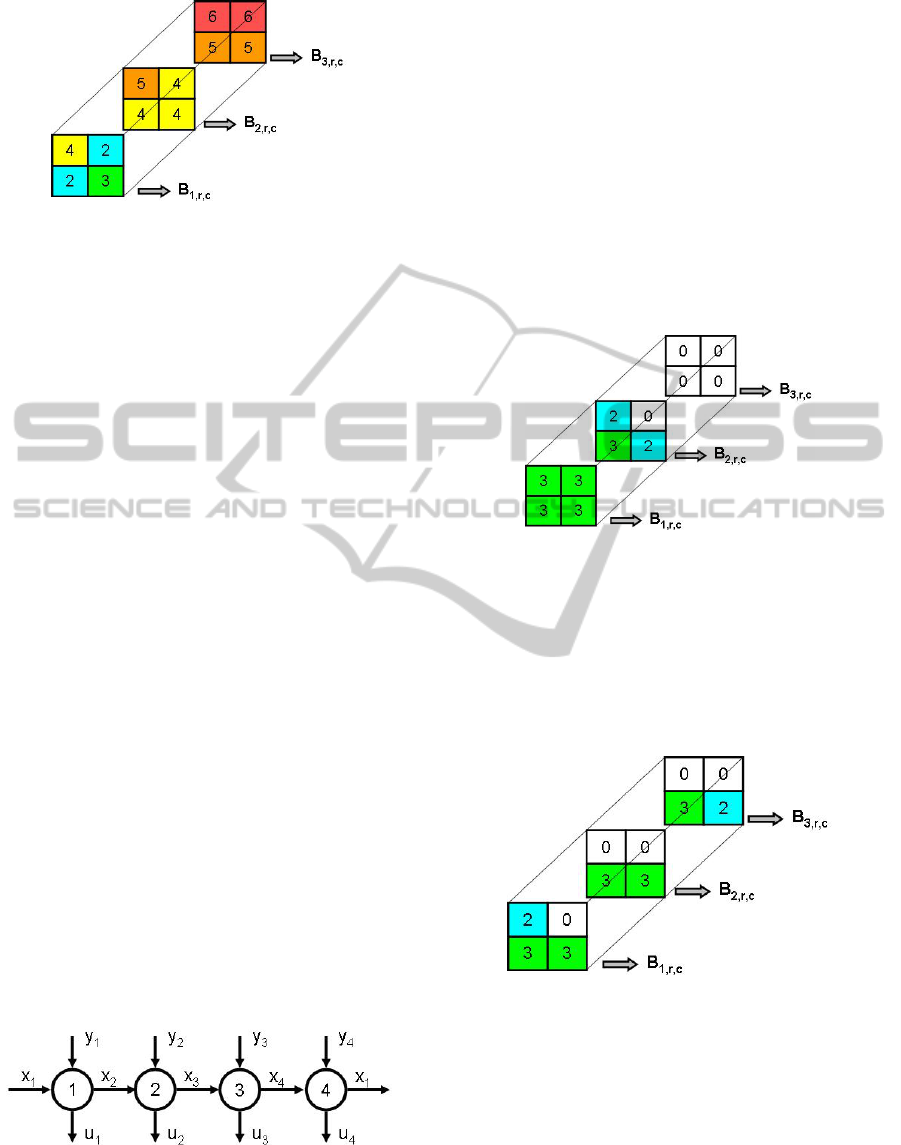
Figure 3: The state matrix B representing a Container ship

occupation with 12 containers capacity and six-port

destination.

In Figure 3, line 2 represents the bottom of the

container ship and line 1 represents the top of the

container ship. Then, the element (1,1,1) is equal to

4, which means that this cell is occupied by a

container, whose destination is port 4. Using the

same criteria, the element (3,2,2) equals 5 and it

means that this cell is occupied by a container,

whose destination is port 5.

Supposing that matrix B in Figure 3 represents

the container ship in port 2, in order to unload this

container ship, it is necessary to move the containers

located in cells (1,2,1), and (1,1,2). However,

observe that the container in cell (1,2,1) can only be

unloaded if the container located in cell (1,1,1) is

unloaded too; even the destination of this container

is port 4. The objective of the CLPP is to minimize

the number of movements of this kind by

performing an adequate arrangement of the

container ship bay for every port.

The representation by rules approach treats the

CLPP as a problem where a matrix B represents the

container ship arrangement (x

) before arriving in

port p and it will be modified in each port by

deciding how to perform the unloading (u

) and

loading operations (y

) by defining an unloading and

a loading rule, respectively. It is also important to

stress that the constraint (2) connects decisions

through ports. The choice of unloading or loading

rule for port 2 can indirectly influence the container

ship arrangement in the port 4, as showed in Figure

Figure 4: The graph representation for the CLPP with four

ports destination.

Next, a description of how the loading and

unloading rules affect the Container ship

arrangement will be presented by supposing that

Container ship dimensions are the same used in

Figure 3.

3.1 Loading Rules

Loading Rule Lr1: This rule fills matrix B row by

row, from left to right, starting from the last line for

each bay in a manner that the containers with the

farthest destination are placed on the lowest part of

the stacks. Figure 5 shows the load rule application

for the container ship in port 1.

Figure 5: The state matrix B representing a Container ship

occupation after applying the Lr1.

Loading Rule Lr2: This rule fills matrix B row by

row, from left to right, starting from the first bay in a

manner that the containers with the farthest

destination are placed on the lowest part of the

stacks. Figure 6 shows the load rule application for

the container ship in port 1.

Figure 6: The state matrix B representing a Container ship

occupation after applying the Lr2.

Loading Rule Lr3: This rule is the reverse of the

Lr1, in other words, fills matrix B row by row, from

right to left, starting from the last line for each bay

the in a manner that the containers with the farthest

destination are placed on the lowest part of the

stacks. Figure 7 shows the load rule application for

the container ship in port 1.

ICORES 2012 - 1st International Conference on Operations Research and Enterprise Systems

136

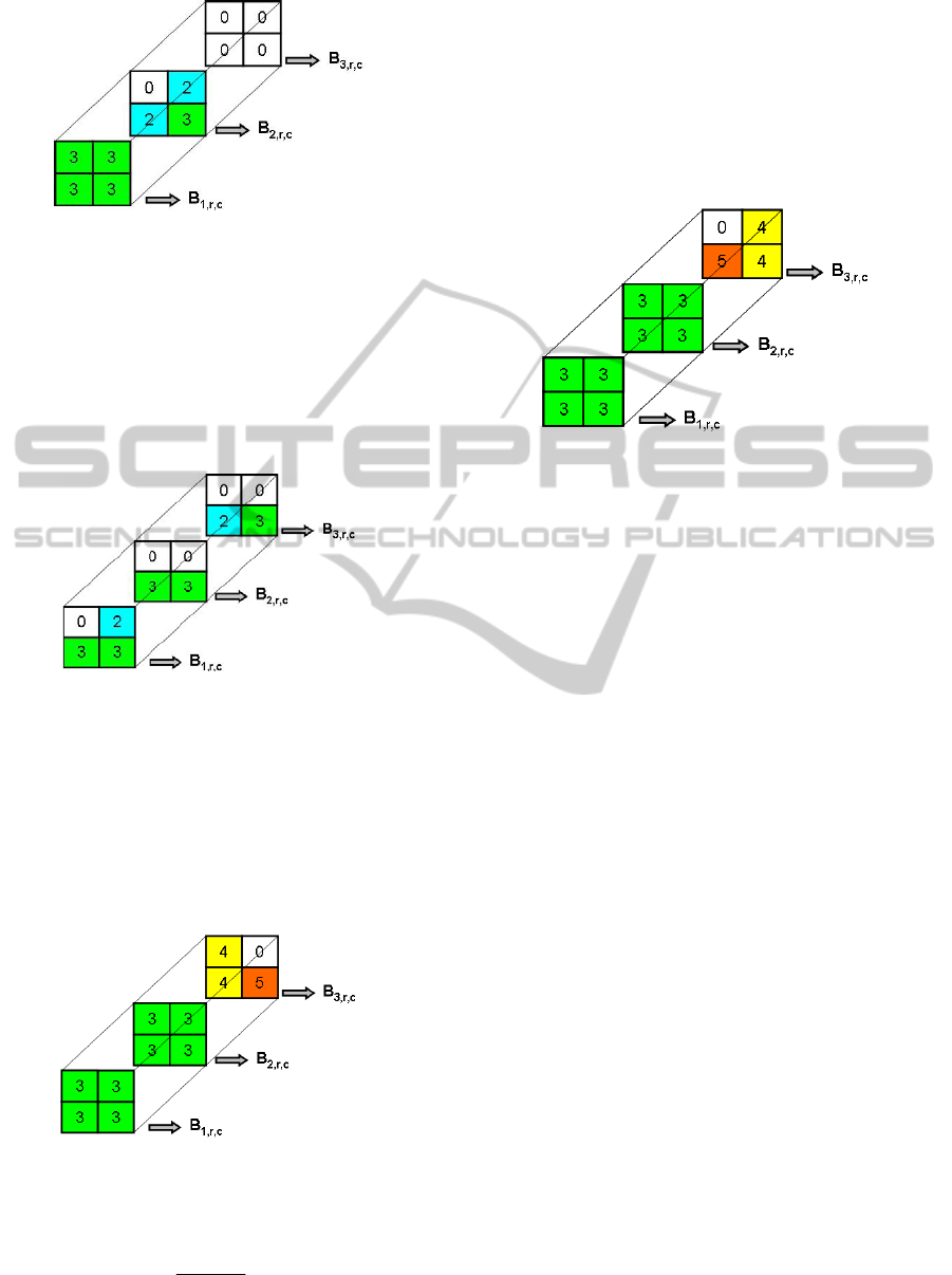
Figure 7: The state matrix B representing a Container ship

occupation after applying the Lr3.

Loading Rule Lr4: This rule is the reverse of the

Lr2, in other words, fills matrix B row by row, from

right to left, starting from the first bay in a manner

that the containers with the farthest destination are

placed on the lowest part of the stacks. Figure 8

shows the load rule application for the container ship

in port 1.

Figure 8: The state matrix B representing a Container ship

occupation after applying the Lr4.

Loading Rule Lr5: This rule fills matrix B from left

to right starting from the first bay row by row until

the row

is reached. The value

is computed by

Eq. (9). Then another bay is filled in a manner that

the containers with the nearest destination are used

on first the stacks. Figure 9 shows this load rule with

the Container ship in port 2.

Figure 9: The state matrix B representing a Container ship

occupation after applying the Lr5.

⎥

⎤

⎢

⎡

∑∑

=+=

(9)

Loading Rule Lr6: This rule is the reverse of the

Lr5, in other words, it fills matrix B from right to

left starting from the first bay row by row until the

row

is reached. The value

is computed by Eq.

(9). Then another bay is filled in a manner that the

containers with the nearest destination are used on

first the stacks. Figure 10 shows this load rule with

the Container ship in port 2.

Figure 10: The state matrix B representing a Container

ship occupation after applying the Lr6.

3.2 Unloading Rules

Unloading Rule Ur1: Suppose that the container

ship arrived at port p. This rule will only remove the

containers whose destination is port p, and all the

ones that are blocking the stacks.

Unloading Rule Ur2: This rule imposes that the

Container ship must unload every container when

arriving at a specific port p, in a manner that it

allows a complete rearrangement of every stack.

3.3 Combining Loading and Unloading

Rules

In order to avoid the need of using two values to

indicate what loading and unloading rules will be

used for every port it is possible to simplify the

encoding by defining the various combinations of

the loading and unloading rules. A particular

combination of the loading and the unloading rules,

for port p, is defined as a rule. For better illustrating

the rule concept, 6 loading rules (LR) and 2

unloading rules (UR) described before can be

combined to generate four rules. Table 1 illustrates

all the rules created as a result of these LR and UR

combination.

SOLVING THE 3D CONTAINER SHIP LOADING PLANNING PROBLEM BY REPRESENTATION BY RULES AND

BEAM SEARCH

137

Table 1: Rules produced by the combination of load and

unload rules.

Load Rules Unload Rules Rule

LR1

UR1 1

UR2 2

LR2

UR1 3

UR2 4

LR3

UR1 5

UR2 6

LR4

UR1 7

UR2 8

LR5 UR1 9

UR2 10

LR6 UR1 11

UR2 12

Table 1 shows the various combinations of LR and

UR forming rules. For example, rule 2 is a

combination of the unload rule UR2 and the load

rule LR1. This encoding allows the representation of

a solution for the CLPP that employs a vector whose

number of elements is equal to the number of ports.

To adopt the encoding described before is

necessary to define a translation scheme which

simulates the unloading and loading actions

proposed by the rules. This translation extract from

every element of the vector s the unload and load

rules that should be applied for the Container ship

arrangement simulation in every port, as described

in Figure 11, and, afterwards, this gives the number

of containers moved in every port.

Translation Scheme

begin

p ← 1,nmov ← 0

start(B)

while (p < N ) do

start

[ur, lr] = extractRules(s(p))

if (p > 1)

[aux, B, T] = unloading(ur, B, p)

nmov ← nmov + aux

end

if (p < N-1)

[aux, B, T] = loading(lr, B, T, p)

nmov ← nmov + aux

end

p ← p + 1

return nmov

end

End

Figure 11: Translation scheme returns number of

containers moved through the ports for a solution vector s.

The translation scheme showed in Figure 11 will

make it easy to employ meta-heuristics and heuristic

methods like the Beam Search described in Section

4 since each solution will be represented by only one

vector and each vector always represents a feasible

solution.

4 THE BEAM SEARCH METHOD

The Beam Search is an implicit enumeration method

for solving combinatorial optimization problems. It

could be said that it is an adaptation of the Branch

and Bound method where only a predetermined

number of best partial solutions (nodes) are

evaluated in each level of the search tree while the

others are discarded permanently. As a big part of

the tree search nodes is discarded, it means that only

a few nodes are kept for further branching and the

others are pruned off permanently, the method

execution time is polynomial in the size of the

problem.

In other words, it can be said that the Beam

Search is a tree search technique that, in each level

of the tree a fixed number of nodes is analyzed, and

thus a fixed number of solutions. The nodes number

analyzed in each level is called beam width and is

denoted by β.

The Beam Search was first used by the

community of Artificial Intelligence to treat

problems of speech recognition (Lowerre, 1976).

The literature gives a lot of applications of this

method in scheduling problems: (Della Croce, F.;

T'kindt, 2002; Dubrovsky et all., 2002; Valente, J.

M. S; Alves, 2005; Ow and Morton, 1988).

Before building the search tree, it is necessary to

establish the following definitions:

(D.1) The tree is constructed by level and in

each level i the assignment of rule r is made for

every port i.

(D.2) The nodes that are in level 1 of the tree are

called seed nodes because each of them will

generate a sub-tree of decisions.

(D.3) In each level i, when making the

assignment a rule r to a port i, two costs are

considered: the unloading number of movements

and the loading number of movements. It is also

important to remember that the rule assignments

performed in previous ports will affect container

ship arrangement in port i which, in turn, indirectly

affect the number of movements in port i.

Considering that the tree has N levels (D.1),

where N is the number of ports, a complete problem

ICORES 2012 - 1st International Conference on Operations Research and Enterprise Systems

138

solution, with attribution of all R rules to all the N

ports is only obtained when defining the assignments

until level N.

To avoid the exponential growth of the tree, the

proposed algorithm does not create all the nodes of

the tree. The nodes are created according to some

rules. In each node of the tree, the following

information is stored as:

(1) Rule Identification;

(2) Port Identification;

(3) Unloading and loading number of container

movements from the simulation (Figure 11) and

related to the allocation made in the node;

(4) Partial cost of the solution, i.e., total number

of movements performed until the actual level was

reached.

During the construction process of the solution

tree, the first criterion whether to create or not a

node in the level i, it must be checked whether the

constraints are within their limits. One node will

only be created (assignment of rule r) in level i, if

the constraints (2) to (6) holds. If not then, all the

branches that will be originated from this node are

not going to exist. However, this is not the case for

the representation by rules integrated with

simulation because the rule r always produces a

feasible arrangement for the container ship in port

(level) i.

After going through the test to check whether the

constraints hold, the node will only remain in the

solution tree if it passes in the search width criterion

β. For example, if the search width chosen by the

user is β =2 in each level, only the nodes that

generate the two minor solutions, computed by the

technique of the greedy algorithm, remain in the

tree.

Thus, for β =2, each node will only generate two

branches, and they will be those that the greedy

solution computation produces the lowest cost.

Initially the algorithm is in level one and start

creating nodes (S1.1). The nodes of level 1 are the

seed nodes and one seed node is created for each

rule. In (S1.2), for each node created in (S1.1), it is

assigned a rule of the vector of rules that will be

applied to each port. Following, it is calculated the

unloading and loading number of movements of

each of these nodes.

The greedy best-first search performed in the 2

Step, aims to choose, in the 3

. Step, which nodes of

level i should remain in the tree of feasible solutions

to respect the width of search β. For example, if

β=2, only two nodes will remain in each level.

The creation process of the greedy solution is

similar to the process of the tree of solutions

creation, except that here, in each step, it is chosen

the allocation that generated the best partial solution

of the node, i.e., the nodes with less costs will be

part of the solution. A more complete description of

the Beam Search Method and also the greedy best-

first search could be found in (Ribeiro et al, 2010).

5 RESULTS

To verify the developed Beam Search performance,

15 instances were automatically and randomly

generated to test the developed approach. These

instances are classified according to the number of

ports, the type of transportation the matrix T, and

Container ship dimension. For each instance, it was

generated a transport matrix T which ensures that the

Container ship capacity will not be exceeded for

every port p. In other words, the value given by Eq.

(9) must be lower or equal to R for every port p. It

means, in mathematical terms, that the inequality

(10) holds for every port.

CRT

×≤

∑∑

=+=11

for all p= 1, ..., N (10)

According to (Avriel et al. 1998), it is possible to

generate three types of transportation matrix: 1 -

Mixed, 2 - Long, 3- Short. This classification for the

transportation matrix expresses how long a container

must be taken by the container ship through the

ports. The Short Transportation Matrix indicates the

majority of the containers that will remain for a short

number of ports until the unloading. For the Long

Transportation Matrix, it is expected the greatest

number of containers remaining in the Container

ship along most of the ports. The Mixed is created in

a manner that it mixes Short and Long instances

characteristics. The ship dimension adopt for the

instances presented in this article are D = 5, R = 6, C

= 50. All instances are available at following site:

https://sites.google.com/site/projetonavio/home

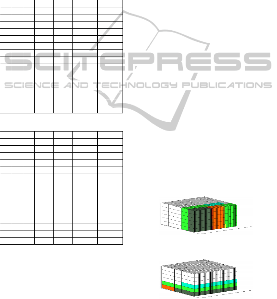
In Tables 2 and 3, the column index I

corresponds to instance number, N corresponds to

how many ports the Container ship has to pass

through, the column index M refers to the type of

transportation matrix, NMin refers to lower bound

on the number of movements (the lower bound value

can be obtained by multiplying by two the sum of

, which comes from Eq. (10)), FO1 is the total

number of movements performed (Eq. (7)), FO2 is

SOLVING THE 3D CONTAINER SHIP LOADING PLANNING PROBLEM BY REPRESENTATION BY RULES AND

BEAM SEARCH

139

total measure of instability (Eq. (8)) and T is the

computational time spent in seconds. The results

presented in Table 2 and 3 were obtained with a

program created in a Matlab 7.0, a machine with a

Processor Intel Core Duo 1.66 GHz, RAM memory

of 2 GB and Operational System Windows Vista

with Service Pack 2.

Table 2: Results obtained for (α=1, β=0).

I N M Nmin

FO1 FO2 T

1 10 1 6994

7072 13625.36 429.46

2 10 2 4172

4202 10300.00 403.39

3 10 3 17060

17074 23009.21 453.83

4 15 1 9974

10234 7234.84 1752.34

5 15 2 4824

4936 18706.99 1550.85

6 15 3 24908

24992 35435.61 1808.89

7 20 1 10262

10432 10432.02 4275.94

8 20 2 4982

5152 18453.41 3946.33

9 20 3 32602

32610 66610.44 4102.06

10 25 1 11014

11154 18180.85 8217.97

11 25 2 5002

5156 27224.53 7576.42

12 25 3 43722

43942 66329.68 9506.44

13 30 1 11082

11430 15023.16 15756.15

14 30 2 4720

5598 8801.76 14468.23

15 30 3 53592

53896 85059.37 17335.38

Table 3: Results obtained for (α=0, β=1).

I N M Nmin

FO1 FO2 T

1 10 1 6994

10432 2630.06 507.34

2 10 2 4172

7172 339.74 522.42

3 10 3 17060

17642 9598.45 618.38

4 15 1 9974

15058 1756.12 2872.77

5 15 2 4824

9560 2312.91 2274.02

6 15 3 24908

25952 17753.68 2022.22

7 20 1 10262

16374 5743.22 5723.36

8 20 2 4982

8652 1678.77 4863.09

9 20 3 32602

33544 44019.80 4651.98

10 25 1 11014

14058 4294.59 9684.85

11 25 2 5002

10240 6163.01 9455.98

12 25 3 43722

45304 31493.30 10397.03

13 30 1 11082

18972 3439.41 18073.31

14 30 2 4720

7544 1050.04 15066.07

15 30 3 53592

55062 38160.15 18301.89

The results presented in Table 2 and 3 shows that

the Beam Search combined with the representation

by rules could provide solutions for instances with

30 ports and a container ship with 5 bays, 6 rows

and 50 columns dimension which, through equations

(1)-(8), each solution must have 40,545,000 binary

variables (30

× 5 × 6 × 50 + 30 × 5 × 6 × 50).

From Tables 2 and 3 is could be said that each 5

increment in the number of ports will results in a

corresponding increment of about 6 minutes in the

computational time spent.

The results also show that when the objective

function is to minimize the number of movements

performed (α=1, β=0), for the Short transportation

matrix (type 3), the representation by rules and the

Beam Search produces results near the optimal

solution in terms of the number of movements,

indicating the adequacy of the proposed rules and

produces results near the lower bound like in the

instances with 10, 15 and 20 ports which solution

are 0.08%, 0.34% e 0.02%, respectively, upper the

lower bound.

For instances with other transportation matrix

like Mixed (type 1) and Long (type 2), the Beam

Search presented results distant from the lower

bound and one possible explanation is the need to

create more adequate rules for these kinds of

instances.

When the objective function is set to minimize

the instability measure (α=0, β=1), the solutions

given by Beam Search has a significant increment in

the number of movements, but with a correspondent

improvement in the instability measure. For

example, for the instance I = 14 the instability

measure is significantly improved and is reduced

about 8 times.

This proves bi-objective optimization nature of

the 3D CLPP and future work must address this

problem with methods that deals with pareto-optimal

frontier in order to choose the solutions.

In order to exemplify the bi-objective

optimization nature of the 3D CLPP the Figure 12

and 13 shows the Container ship arrangement for the

best solutions found for instance I = 1 when the

weights are set as (α=1, β=0) and (α=0, β=1),

respectively.

Figure 12: The Container ship occupation in port 2 for the

better solution found with (α=1, β=0).

Figure 13: The Container ship occupation in port 2 for the

better solution found with (α=0, β=1).

ICORES 2012 - 1st International Conference on Operations Research and Enterprise Systems

140

6 CONCLUSIONS AND FUTURE

WORK

This Article shows, for the first time, a new

representation for the 3D Container ship loading

planning problem (3D CLPP) that has the following

advantages:

• It allows a compact encoding by representing

the solution as a vector with P elements instead of

(R x C) x ( P+P

) binary variables, which enables a

large-scale problem solving.

• The skilled personnel experience can be

incorporated in the optimization process under the

form of a rule and a computational simulation.

• The solutions with this encoding are always

feasible, which avoids the problem of processing

time consumption to make solutions feasible.

This new encoding gives great savings in

computational time and produced solutions with

good quality, and, in some instances, the optimality

is reached or almost reached, showing that this

approach is promising.

One promising idea for future work is to codify

in the form of rules the previous approaches

proposed for the Container ship problem.

Other idea is that future work must address this

3D CLPP with methods that deals with pareto-

optimal frontier in order to choose the solutions

ACKNOWLEDGEMENTS

This research was supported by the Foundation for

the Support of Research of the State of São Paulo

(FAPESP) under the process 2010/51274-5 and

Brazilian Council for the Development of Science

and Technology (CNPq). Also, the authors would

like to thank the anonymous reviewer for their

valuable comments, which helped to clarify and

improve the contents of this paper.

REFERENCES

Ambrosino, D.; Sciomachen A.; Tanfani, E., 2006. A

decomposition heuristics for the container ship

stowage problem, J. Heuristics, v.12, p. 211–233.

Ambrosino, D., Anghinolfi, D., Paolucci, M., Sciomachen,

A., 2010. An Experimental Comparison of Different

Heuristics for the Master Bay Plan Problem. In SEA,

314-325.

Avriel, M.; Penn, M., 1993. Container ship stowage

problem, Computers and Industrial Engineering, v. 25,

p. 271-274.

Avriel, M.; Penn, M.; Shpirer, N.; Wittenboon, S., 1998.

Stowage planning for container ships to reduce the

number of shifts, Annals of Operations Research, v.

76, p. 55-71.

Avriel, M.; Penn, M.; Shpirer, N., 2000. Container ship

stowage problem: complexity and connection to the

coloring of circle graphs, Discrete Applied

Mathematics, v. 103, p. 271-279.

Della Croce, F.; T'kindt, V., 2002. A Recovering Beam

Search Algorithm for the One-Machine Dynamic Total

Completion Time Scheduling Problem, Journal of the

Operational Research Society, vol 54, pp. 1275-1280.

Dubrovsky, O.; Levitin, G., Penn, M., 2002. A Genetic

Algorithm with a Compact Solution Encoding for the

Container Ship Stowage Problem, Journal of

Heuristics, v. 8, p. 585-599.

Lowerre, B. T.; 1976. The HARPY Speech Recognition

System, PhD. thesis, Carnegie-Mellon University,

USA, 1976.

Ow, P. S, Morton, T. E., 1988. Filtered Beam Search in

Scheduling, International Journal of Production

Research, vol. 26, pp. 35-62.

Ribeiro, C. M., Azevedo, A. T., Teixeira, R. F., Problem

of Assignment Cells to Switches in a Cellular Mobile

Network via Beam Search Method, WSEAS

Transactions on Communications, vol 1, pp. 11-21,

2010.

Valente, J. M. S; Alves, R. A. F. S., 2005. Filtered and

Recovering Beam Search Algorithm for the

Early/Tardy Scheduling Problem with No Idle Time,

Computers & Industrial Engineering, vol. 48, pp. 363-

375, 2005.

Wilson, I.; Roach, P. Container stowage planning: a

methodology for generating computerised solutions,

Journal of the Operational Research Society, v. 51, p.

1248-1255, 2000.

SOLVING THE 3D CONTAINER SHIP LOADING PLANNING PROBLEM BY REPRESENTATION BY RULES AND

BEAM SEARCH

141