SOLVING THE RCPSP WITH AN EVOLUTIONARY

ALGORITHM BASED ON INSTANCE INFORMATION

José António Oliveira, Luís Dias and Guilherme Pereira

Centre ALGORITMI, University of Minho, Braga, Portugal

Keywords: Optimization, Project Management, Scheduling, RCPSP, Metaheuristics, Genetic Algorithm, Random Keys.

Abstract: The Resource Constrained Project Scheduling Problem (RCPSP) is NP-hard thus justifying the use meta-

heuristics for its solution. This paper presents an evolutionary algorithm developed for the RCPSP problem.

This evolutionary algorithm uses an alphabet based on random keys that makes easier its implementation

while solving combinatorial optimization problems. Random keys allow the use of conventional genetic

operators, what makes easier the adaptation of the evolutionary algorithm to new problems. To improve the

method's performance, this evolutionary algorithm uses an initial population that is generated considering

the information available for the instance. This paper studies the impact of using that information in the

initial population. The computational experiments presented compare two types of initial population - the

conventional one (generated randomly) and this new approach that considers the information of the

instance.

1 INTRODUCTION

The Resource Constrained Project Scheduling

Problem (RSPSP) is a classic project scheduling

problem, and belongs to the set of Combinatorial

Optimization (CO) problems that are very hard to

solve and therefore require heuristic procedures. The

use of exact methods to solve this type of CO

problems is limited to small size instances. The

RCPSP problem is a generalization of the

production-specific Job-Shop Scheduling Problem

(JSSP). According to (Zhang et al., 2007), the

Branch and Bound methods for JSSP do not solve

instances larger than 250 operations within a

reasonable time. As stated in (Liu et al., 2008), in

practical manufacturing environments, the scale of

job shop scheduling problems could be much larger

- in some big textile factories, the number of jobs

can be as much as 1,000.

Heuristic methods became very popular and have

gained success in solving scheduling problems. For

the last twenty years, a huge quantity of papers have

been published presenting several metaheuristic

methods. From Simulated Annealing to Particle

Swarm Optimization (Lian et al., 2006), there are

several variants of the same class of method. A very

popular method among researchers is the

Evolutionary Algorithms (EA).

Vaessens et al. (1996) presented the Genetic

Algorithms as the less effective metaheuristic to

solve the JSSP. A possibility to increase the

efficiency and the effectiveness on an algorithm is to

include in the algorithm specific knowledge of the

problem. Several works include some specific local

search for the JSSP that is based in the critical path

of a disjunctive graph. This work presents a strategy

to improve the effectiveness and efficiency of an

Evolutionary Algorithm to solve the RCPSP. Once

verified the difficulty to solve the RCPSP changes

from instance to instance, a procedure can be

implemented to get knowledge from the instance and

transfer it to the EA's initial population. The

developed EA is based in a previous one, developed

by us, to the JSSP (Oliveira et al., 2010) according

to the similarities between both problems. Above all

of this, the strategy to enhance the effectiveness was

tested in the JSSP by Oliveira et al. (2010) and in a

very particular case it improves the makespan in

about 8%.

The paper is organized as follows: an

introductory section defines the RCPSP problem and

its representation with the use of an AoN graph; a

central section describes the methodology and a

numerical example that supports the explanation of

the constructive algorithm; finally, some conclusions

and a discussion on future work are presented.

157

António Oliveira J., Dias L. and Pereira G..

SOLVING THE RCPSP WITH AN EVOLUTIONARY ALGORITHM BASED ON INSTANCE INFORMATION.

DOI: 10.5220/0003759401570164

In Proceedings of the 1st International Conference on Operations Research and Enterprise Systems (ICORES-2012), pages 157-164

ISBN: 978-989-8425-97-3

 2012 SCITEPRESS (Science and Technology Publications, Lda.)

2 RCPSP

A project can be represented as a network of n

activities in a graph, where exist links between pairs

of activities, representing processing precedence

between them. The order to process the set of

activities must respect the precedence set. There are

two ways to represent a project: the activity-on-arc

(AoA) and the activity-on-node (AoN).

In the AoA mode, the set of nodes represents the

"events" (start/end processing) and the set of arcs

represents the "activities." In the AoN scheme, the

set of nodes represents the "activities" and the set of

arcs represents the precedence between the

"activities." In general, each activity requires the

simultaneous use of several resources

(Demeulemeester et al., 2003). In this paper, the

AoN scheme has been adopted since it allows a

direct correspondence with the disjunctive graph that

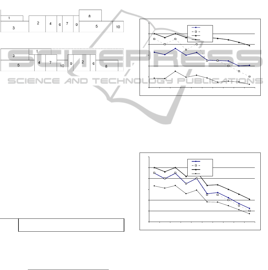
is usually used to represent the JSSP. Figure 1 shows

a project network with 10 activities, represented in a

AoN scheme (Ranjbar and Kianfar, 2009).

Figure 1: AoN project network.

For a given r renewable resources R1,..,Rr, a

constant amount of bk units of resource Rk is

available at any time. Activity j must be processed

for dj time units, where preemption is not allowed.

During this period of time, a constant amount of rjk

units of resource Rk is occupied. The objective is to

determine the starting times of Sj for the activities

j = 1,..,n in a way that:

i) at each time t, the total resource demanded is

less than or equal to the resource availability

for each resource type;

ii) the given precedence constraints are fulfilled;

iii) the makespan

max 1

max

, where

jjj

CSd=+

, is minimized.

Figure 1 shows also 2 dummy activities, node 0

and node 11 which represent the starting time of the

project (node 0) and the project conclusion time

(node 11). Their duration is null. Each node shows

the duration of the activity and the amount of

renewable resources. In this project instance it is

considered only one renewable resource. The set of

arcs represent the precedence set of the project.

Activity 6 can only be started after activities 1 and 2

are completed.

The RCPSP is a highly complex optimization

problem due to its combinatorial nature. This

problem belongs to the NP-hard class (Brucker et

al., 1998), and so an efficient algorithm for obtaining

exact solutions is unknown.

The research on the RCPSP has been extensive

along the years and it involves exact algorithms and

heuristic methodology. Generally, the exact methods

are based on branch and bound algorithm, where the

branch strategies are related to the choice of

activities in the disjunctive graph that represents the

project. Also, in this field of research, the continuous

development of new and better lower bounds for the

optimal solution is pointed out, what is a

fundamental auxiliary information for the heuristic

methods.

The state-of-the-art RCPSP performed by

Hartmann and Kolisch (2000) and updated later

(Kolisch and Hartmann, 2006) shows a bigger

number of publications on heuristics than on exact

methods. In this study, the authors explain that, in

the specialized bibliography, there are several

heuristic methodologies to deal with RCPSP. These

methods can be classified as “single pass” (over

activities set) or “multiple pass”, based in priority

dispatch rules to construct the solution, local

iterative improvement and meta-heuristics.

In the metaheuristics set, several approaches

have arisen, such as: evolution strategies, taboo

search, ant colony system, variable neighbourhood

search and simulated annealing. Some of those

metaheuristics include hybridization with local

search procedures and with single pass or multiple

pass. An example of hybridization is given by

Ranjbar and Kianfar (2009). They presented a

hybrid metaheuristic algorithm for solving the

RCPSP, which contains a scatter search skeleton and

uses a special solution combination method for

making children.

The process to construct a solution is a

fundamental component in the heuristic

methodology. With RCPSP in particular, this

component is called Schedule Generation Scheme

(SGS). For the RCPSP, two SGS models exist: the

serial model and the parallel model. It is possible to

find in the literature heuristic procedures that use

ICORES 2012 - 1st International Conference on Operations Research and Enterprise Systems

158

either one scheme or the other, but it is also possible

to find some methodologies that use both, or even a

combination of the two models.

Analyzing the computational results presented in

the literature performed with test instances with 30,

60 and 120 activities, it is possible to point out that

the better approximation methodology is the

population-based heuristic with representation of list

of activities and serial SGS. The parallel SGS seems

to be better when dealing with large instances.

It seems that further research for approach

methods will concentrate on the development of

algorithms which integrate the Forward–Backward

Improvement strategy (FBI), since four of the best

six heuristics already use this local search strategy.

The FBI strategy has two phases: the first phase

gives a feasible schedule using a priority dispatch

rule to sequence the activities in a bidirectional way;

the second phase tries to improve the resources

assignment performing successive bidirectional

passes without increasing the project duration

obtained in the first phase.

The performance of a heuristic can be improved

by integrating specific knowledge of the problem.

With the RCPSP, the integration of a constructive

algorithm in an Evolutionary Algorithm (EA)

constructs only active schedules. This strategy is

implemented similarly to that performed for the

particular case of the Job Shop Scheduling Problem.

3 EVOLUTIONARY ALGORITHM

This work adopts a method based on Evolutionary

Algorithms. EA can be viewed as a metaheuristic

search techniques that imitates the principle of

evolution in nature i.e., EAs use a set of competing

potential solutions of the problem which evolve

according to rules of selection and transformation.

It is possible to briefly describe the functioning

of an EA in the following way. An EA proceeds in

iterations called generations. In each generation, a

set of solutions called population is generated.

Usually, the first population is generated randomly.

A new population is generated from a current

population using selection and transformation

operators. The members of a population are called

individuals. The fitness-function assigns a value

called fitness to each individual. Given an individual

and its fitness, a selection operator decides if an

individual from the current population is used as an

input of a transformation operator. A transformation

operator creates a new element of a new population

from an arbitrary number of elements of the current

population. It is expected that during the search

process, increasingly better solutions are found. To

achieve this goal, it is necessary that the

transformation operators focus attention on high

fitness. Very common transformation operators are

reproduction (copying an individual to the new

population unaltered), mutation (an individual is

changed in a random fashion) and crossover (where

parts of two individuals are combined).

The simplicity of an EA to model more complex

problems and its easy integration with other

optimization methods were factors that were

considered for its choice. One advantage of this EA

is the portability to other problems. The algorithm

proposed was conceived to solve the RCPSP, but the

method can be adapted to solve other variants or

extensions of the RCPSP, such as the RCMPSP. In

fact, the EA was already adapted to solve other type

of problems in the Project Planning field (Silva et

al., 2010). When implementing an appropriate

algorithm to construct solutions based on

chromosome, the EA can also solve other scheduling

algorithms like job shop (Oliveira et al., 2010).

Furthermore, random keys chromosome (Bean,

1994) also enables to apply the algorithm in other

type of problems once conventional genetic

operators, which are problem independent, could be

used.

As Gonçalves et al. (2005) state, the important

feature of random keys is that all offspring formed

by crossover are feasible solutions, when it is used

as a constructive procedure based on the available

operations to schedule and the priority is given by

the random key allele. Through the dynamics of the

genetic algorithm, the system learns the relationship

between random key vectors and solutions with

good objective function values.

A chromosome represents a solution to the

problem and is encoded as a vector of random keys

(random numbers). In this work, according to Cheng

et al. (1996), the problem representation is indeed a

mix from priority rule-based representation and

random keys representation. An excellent

classification of heuristics algorithms for the RCPSP

was provided by Kolisch and Hartmann (1999).

They discussed several methods and alternatives to

generate different type of solutions for the RCPSP

and, in particularly, they provided detailed

algorithms to generate active schedules. In the

meantime, in this EA the solutions are decoded /

constructed by an algorithm, that is based on Giffler

and Thompson’s algorithm (Giffler and Thompson,

1960) for the JSSP. While the Giffler and

Thompson’s algorithm can generate all the active

SOLVING THE RCPSP WITH AN EVOLUTIONARY ALGORITHM BASED ON INSTANCE INFORMATION

159

plans for the JSSP, the adapted constructive

algorithm only generates a plan according to the

chromosome. Similar to the JSSP, the solutions of

RCPSP can be classified on three sets: Semi-active,

Active, and Non-delay schedules (Sprecher et al.,

1995).

As advantages of this strategy, we have pointed

the minor dimension of solution space, which

includes the optimum solution and the fact that it

does not produce impossible or disinteresting

solutions from the optimization point of view. On

the other hand, since the dimensions between the

representation space and the solution space are very

different, this option can represent a problem

because different chromosomes can represent the

same solution.

Using the adapted Giffler and Thompson’s

algorithm to construct a solution based on the

priority values of each activity, a Serial Schedule

Generation Scheme is adopted. It has been shown by

Kolisch (1996) that a serial scheme yields better

results when a large number of schedules is

computed for one project instance. Attending

Hartmann (1998), the parallel scheme might exclude

all optimal solutions from the search space, while

the search space of the serial scheme always

contains an optimal schedule.

The constructive algorithm has n stages and in

each stage an activity is scheduled. To assist the

algorithm’s presentation, consider the following

notation existing in stage t:

P - the partial schedule of the

(

)

1t −

scheduled

activities;

S - the set of activities schedulable at stage t , i.e.

all the activities that must precede those in

are in

P ;

Q - the set of activities queued at stage t , i.e. all

the activities that are not in

S nor in

P ;

- the earliest time that activity

a in

S could be

started;

- the earliest time that activity

a in

S could be

finished, that is

kkk

;

∗

- the set of resources used by

a in

S which

has

{

}

min

aS k

∗

∈

;

∗

- the conflict set formed by

a in

S which use

at least one resource of

∗

and

∗

< ;

∗

- the selected activity to be scheduled at stage t .

Table 1 presents the constructive algorithm that

is used to build a solution.

In Step 3, instead of using a priority dispatching

rule, the information given by the chromosome is

used. If the maximum allele value is equal for two or

more operations, one is chosen randomly.

Table 1: A constructive algorithm.

3.1 First Generation

In the RCPSP it is possible to calculate for each

activity the remaining time for completion of the

project. In the project network this time is referred to

as “tail”. This value represents the longest path from

the activity to node n+1. It is easy to admit that the

activities with large tail must be sequenced first

because they could define the makespan. Indeed,

there exists the dispatching rule that is used in

practice JSSP which sequences operations in first

place that belongs to the job with Most Work

Remaining (MWR).

Consider the following example presented in

Figure 1, with ten activities. In this instance there is

only one constrained renewable resource with 4

available units. Table 2 presents this instance. The

activities are numbered sequentially and represented

by index j. The duration of each activity is given in

the row “duration”.

Table 2: The instance data.

Activity 12345678910

duration 4352612432

resources 1323233212

tail 9897855432

Step 1

Let

with

being null.

will be the

set of all activities with no predecessors.

Step 2

Find

{

}

min

aS k

∗

∈

and identify

∗

Form

∗

Step 3

Select activity

∗

, with the greatest

allele value.

Step 4

Move to next stage by

(1)

adding

∗

, so creating

;

(2) removing

∗

from the list of

predecessors of activities in

deleting

∗

from

and creating

by adding to

the activities

that

∗

as the only predecessor;

(3)

deleting

∗

from

and creating

by adding to

the activities

with no predecessors;

(4)

incrementing

by 1.

Step 5

If there are any activities left

unscheduled

(

)

tN<

, go to Step 2.

Otherwise, stop.

ICORES 2012 - 1st International Conference on Operations Research and Enterprise Systems

160

The tail row shows the remaining time to

complete the project including the processing of the

activity. For instance, the tail of activity 3 is 9 and is

equal to the duration of activities 3, 8 and, 11, and

that is respectively 5, 4, and 0 (Figure 1). It

correspond to the longest path from node 3 to node

11.

Applying the MWR rule to this instance the

schedule is given in Figure 2. For this small

example, the optimal solution is presented in Figure

Figure 2: Gantt chart of MWR solution.

Figure 3: Gantt chart of optimal solution.

In the chosen random key representation, a

chromosome is a vector of N genes that are real

numbers between 0 and 1. The representation has

one gene for each activity. Table 3 presents two

chromosomes for a RCPSP of ten activities. The

second chromosome (chrms2) was generated

randomly, while the first chromosome (chrms1)

represents the information that is obtained dividing

in the example above the tail value per maximum

tail value plus one (9+1 in the example). Applying

the constructive algorithm and considering the

chromosome chrms1, the solution of Figure 2 is

obtained. Attending to this property we implement a

procedure to generate the first population that

includes some knowledge about the instance in the

form of the tail of each activity.

Table 3: Chromosomes for a RCPSP10.

Activity

345

910

chrms1

0.90 0.80 0.90 0.70 0.80 0.50 0.50 0.40 0.30 0.20

chrms2

0,30 0.30 0.70 0.80 0.30 0.40 0.20 0.70 0.10 0.20

To generate L individuals in a population the

following expression at (1) is used to generate the

allele value for each gene j:

(

)

;

max( )

randbetween tail tail i GAP

allele

tail i GAP

+×

(1)

3.2 Considerations About GAP

The GAP value allows obtaining at the end of

population a quite random chromosome. The higher

the GAP, the more random is the population. Lower

GAP gives a population close to the MWR dispatch

rule.

For a population of 50 individuals, the graphic

presented in Figure 4 presents some statistics of the

allele values for each gene (10 activities / genes).

The average value, maximum value, minimum value

and also the tail value of each operation is presented.

0,00

0,20

0,40

0,60

0,80

1,00

1,20

12345678910

average

tail

max

min

Figure 4: Statistics of allele’s values.

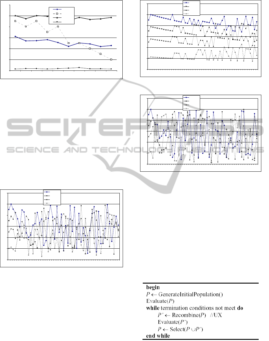
Figures 5 and 6 show the GAP effect in the

statistics of the allele values for the 10 activities.

Figure 5 shows the statistics when a small GAP is

used. The values are very close to the tail of each

operation.

0,00

0,20

0,40

0,60

0,80

1,00

1,20

12345678910

average

tail

max

min

Figure 5: Statistics of allele’s values with small GAP.

Figure 6 shows the statistics for a high GAP. The

range of variation for the alleles is very similar for

all genes, so the population is “more random”.

SOLVING THE RCPSP WITH AN EVOLUTIONARY ALGORITHM BASED ON INSTANCE INFORMATION

161

0,00

0,20

0,40

0,60

0,80

1,00

1,20

12345678910

average

tail

max

min

Figure 6: Statistics of allele’s values with high GAP.

Figure 7 presents the alleles’ values of four genes

when using a GAP=2. These genes belong to the

activities having different tails values which are

respectively 9, 7, 5, and 2. It is possible to verify that

for the first chromosomes the alleles’ values

translate the priority give by the tail of each

operation. It is also possible to verify that the last

individuals have quite random alleles. It is possible

to see that in some individuals the activity 10

(Gene10) and activity 6 (Gene6) have a priority

greater than the activity 1 (Gene1). This situation

allows a first sequence of these activities before

activity 1, which is the activity with the greatest tail.

0,2

0,4

0,6

0,8

1,2

1 3 5 7 9 111315171921232527293133353739414345474951

Gene1

Gene4

Gene6

Gene10

Figure 7: The allele generation.

Figures 8 and 9 show the effect of GAP on the

allele generation for the same genes. Figure 8 shows

the alleles values when used as small GAP. The

values are very close to the tail of each operation.

Figure 9 shows the statistics for a high GAP. The

range of variation for the alleles is very similar for

all genes, so these allow “any” sequence to schedule

these four activities.

0,2

0,4

0,6

0,8

1,2

1 3 5 7 9 111315171921232527293133353739414345474951

Gene1

Gene4

Gene6

Gene10

Figure 8: The allele generation with small GAP.

0,2

0,4

0,6

0,8

1,2

1 3 5 7 9 111315171921232527293133353739414345474951

Gene1

Gene4

Gene6

Gene10

Figure 9: The allele generation with high GAP.

3.3 The Algorithm Structure

The genetic algorithm has a very simple structure

and can be represented in Table 4. It begins with

population generation and her evaluation. Attending

to the fitness of the chromosomes the individuals are

selected to be parents. The crossover is applied and

it generates a new temporary population that also is

evaluated. Comparing the fitness of the new

elements and of their progenitors the former

population is updated.

Table 4: Genetic algorithm.

The Uniform Crossover (UX) is used this work.

This genetic operator uses a new sequence of

random numbers and swaps both progenitors' alleles

if the random key is greater than a prefixed value.

ICORES 2012 - 1st International Conference on Operations Research and Enterprise Systems

162

Table 5 illustrates the UX's application on two

parents (prnt1, prnt2), and swaps alleles if the

random key is greater or equal than 0.75.

Table 5: The UX crossover.

910

prnt1

0.89 0.48 0.24 0.03 0.41 0.11 0.24 0.12 0.33 0.30

prnt2

0.83 0.41 0.40 0.04 0.29 0.35 0.38 0.01 0.42 0.32

randkey

0.64 0.72 0.75 0.83 0.26 0.56 0.28 0.31 0.09 0.11

dscndt1

0.89 0.48 0.40 0.04 0.41 0.11 0.24 0.12 0.33 0.30

dscndt2

0.83 0.41 0.24 0.03 0.29 0.35 0.38 0.01 0.42 0.32

The genes 3 and 4 are changed and it originates

two descendants (dscndt1, dscndt2). Descendant 1 is

similar to parent 1, because it has about 75% of

genes of this parent.

4 EXPERIMENTS

The Genetic Algorithm was coded in C++ and the

computer used was a PC Pentium IV 3GHz

processor with 1024 Mbytes of RAM., with Linux

operative system.

The problem data set was taken from PSPLIB

datasets (Kolisch and Sprecher, 1997). The dataset

consists of four test sets J30, J60, J90 and J120 that

contain problem instances of 30, 60, 90 and 120

activities, respectively, and have been constructed

by the instance generator ProGen. In this

preliminary study we present results for 4 instances

with 30 activities: J301_1, J301_2, J301_3 and

J301_4. The optimal value for these instances are

respectively 43, 47, 47 and 62.

Table 6 resumes the computational experiments.

For each instance were made five runs considering

the tail information on the initial population, and

also were made five runs with an initial population

generated randomly. In each run the algorithm

performs 5000 iterations.

Table 6 shows the average value and the best

value of five runs. Each column shows the values in

different iterations of the algorithm. In the

computation experiments it was only used a value

for the GAP.

Globally in all experiments the use of tails’

information of the instance produces in average

1.8% better results. This advantage is more evident

in the initial iterations, so for some instances it was

obtained solutions about 5.5% better. In terms of

best solution the use of tails' information is relevant

on the initial iterations. In some instances the use of

tails information produces a solution about 3.6%

better than using a random initial population.

Table 6: Computational experiments.

Iteration Average Best Average Best

1 76.2 73 76.2 75

50 61.8 60 58.4 58

100 60.8 59 58.4 58

500 57.0 55 54.0 54

1000 56.0 54 54.0 54

2000 55.0 53 53.0 53

5000 53.4 53 53.0 53

J301_1_Random J301_1_tails

Iteration Average Best Average Best

1 89.2 84 90.4 90

50 84.2 84 82.6 81

100 84.0 84 82.6 81

500 80.8 80 78.4 78

1000 80.4 80 78.4 78

2000 78.8 77 78.4 78

5000 78.4 77 78.4 78

J301_2_Random J301_2_tails

Iteration Average Best Average Best

1 93.0 91 89.6 89

50 81.6 81 80.6 79

100 81.0 81 79.8 79

500 78.6 77 79.0 78

1000 76.6 75 76.0 76

2000 76.4 75 76.0 76

5000 75.4 75 76.0 76

J301_3_Random J301_3_tails

Iteration Average Best Average Best

1 152.6 146 149.6 147

50 148.0 146 144.4 143

100 145.4 142 144.4 143

500 140.2 138 136.0 136

1000 139.6 138 136.0 136

2000 139.0 138 136.0 136

5000 137.4 136 136.0 136

J301_4_tailsJ301_4_Random

5 CONCLUSIONS

This paper presents a new method for generating the

initial population for an evolutionary algorithm that

solves the Resource Constrained Project Scheduling

Problem (RCPSP). This proposed method, through

known information for each instance, establishes

different priorities to the activities based on the

remaining processing time to finish the project, thus

generating an initial population. The algorithm uses

a representation based on random keys.

Results are then compared with the conventional

random generation and some promising conclusions

arise. In fact the experimental computation shows

better results when the information of the instance is

used, especially on initial iterations.

Definitely this could be a very simple way to

increase effectiveness of the algorithm. Furthermore

the use of instance information could also be

parameterized, obtaining levels of convergence of

the algorithm depending on available CPU time.

Since the random keys representation has no

Lemarkin property, it is our intention to apply the

SOLVING THE RCPSP WITH AN EVOLUTIONARY ALGORITHM BASED ON INSTANCE INFORMATION

163

same strategy on initial population generation in

other types of representation for the RCPSP, namely

the permutation code.

Further work would also consist on applying this

method to other problems. The Resource

Constrained Multi-Project Scheduling Problem

(RCMPSP), as a generalization of the RCPSP,

would be the next candidate for evaluating the

advantages of the approach presented above.

REFERENCES

Bean, J. C., 1994. Genetics and random keys for

sequencing and optimization. ORSA Journal on

Computing, 6, 154–160.

Brucker, P., Knust, S., Schoo, A., Thiele, O., 1998. A

branch and bound algorithm for the resource-

constrained project scheduling problem. European

Journal of Operational Research, 107, 272-288.

Cheng, R., Gen, M., Tsujimura, Y., 1996. A tutorial

survey of job-shop scheduling problems using genetic

algorithms part I: Representation. Computers &

Industrial Engineering, 34 (4), 983–997.

Demeulemeester, E., Vanhocke, M., Herroelen, W., 2003.

RanGen: A Random Network Generator for Activity-

on-the-node Networks. Journal of Scheduling, 6, 17-

38.

Giffler, B., Thompson, G. L., 1960. Algorithms for

solving production scheduling problems. Operations

Research, 8, 487-503.

Gonçalves, J. F., Mendes, J. J., Resende, M. G. C., 2005.

A hybrid genetic algorithm for the job shop scheduling

problem. European Journal of Operational Research,

167, 77–95.

Hartmann, S., Kolisch, R., 2000. Experimental evaluation

of state-of-the-art heuristics for the resource-

constrained project scheduling problem. European

Journal of Operational Research, 127, 2, 394-407.

Kolisch, R., 1996. Serial and parallel resource-constrained

project scheduling methods revisited: Theory and

computation. European Journal of Operational

Research, 90, 320–333.

Kolisch, R., Hartmann S., 1999. Heuristic algorithms for

solving the resource-constrained project scheduling

problem - Classification and computational analysis,

in Weglarz, J. (Eds.): Project Scheduling – Recent

Models, Algorithms and Applications, Kluwer,

Boston, p. 147 - 178.

Kolisch, R., Hartmann, S., 2006. Experimental

investigation of heuristics for resource-constrained

project scheduling: An update. European Journal of

Operational Research, 174, 1, 23-37.

Kolisch, R., Sprecher, A., 1997. PSPLIB - A project

scheduling library. European Journal of Operational

Research, 96, 205-216.

Lian, Z., Gu, X., Jiao, B., 2006. A similar particle swarm

optimization algorithm for job-shop scheduling to

minimize makespan. Applied Mathematics and

Computation, 183, 1008–1017.

Liu, M., Hao, J., Wu, C., 2008. A prediction based

iterative decomposition algorithm for scheduling

large-scale job shops, Mathematical and Computer

Modelling, 47, 411–421.

Oliveira, J. A., Dias, L., Pereira, G., 2010. Solving the Job

Shop Problem with a random keys genetic algorithm

with instance parameters. Proceedings of 2nd

International Conference on Engineering

Optimization – EngOpt 2010, Lisbon – Portugal.

Ranjbar, M., Kianfar, F., 2009. A Hybrid Scatter Search

for the RCPSP. Transaction E: Industrial

Engineering, 16, 11-18.

Silva, H., Oliveira, J. A., Tereso, A., 2010. Um Algoritmo

Genético para Programação de Projectos em Redes de

Actividades com Complementaridade de Recursos.

Revista Ibérica de Sistemas y Tecnologías de la

Información,. 6, 59-72.

Sprecher, A., Kolisch, R., Drexl A., 1995. Semi-active,

active, and non-delay schedules for the resource-

constrained project scheduling problem, European

Journal of Operational Research, 80, 94-102.

Vaessens, R., Aarts, E., Lenstra, J. K., 1996. Job Shop

Scheduling by local search. INFORMS Journal on

Computing, 8, 302-317.

Zhang, C., Li, P., Guan, Z., Rao, Y., 2007. A tabu search

algorithm with a new neighborhood structure for the

job shop scheduling problem. Computers &

Operations Research, 53, 313-320.

ICORES 2012 - 1st International Conference on Operations Research and Enterprise Systems

164