EVALUATING VEHICLE ROUTING PROBLEMS

WITH SUSTAINABILITY COSTS

Ignacio Eguia, Jesus Racero

and Fernando Guerrero

Department of Management Science, University of Seville, Camino de los Descubrimientoss/n, 41092, Seville, Spain

Keywords: Routing, Green Logistics, Linear Programming, Mathematical Modelling.

Abstract: In this paper, we study the road freight transportation activities, which are significant sources of air

pollution, noise and greenhouse gas emissions, with the former known to have harmful effects on human

health and the latter, responsible for global warming. Specifically, an extension of the classical Capacitated

Vehicle Routing Problem is presented, including realistic assumptions (Time Windows, Backhauls and

Heterogeneous Fleet with different vehicles and fuel types). The decisions are aimed at the selection of

vehicle and fuel types, the scheduling of deliveries and pick-up processes and the consolidation of freight

flows. The classical objective functions of minimizing the total travel distance or the internal costs (driver,

fuel or maintenance) are extended to other sustainable measures: the amount of air pollution and greenhouse

gas emissions, the energy consumption and their costs. A mathematical model is described and an

illustrative example is performed.

1 INTRODUCTION

Environmental issues can impact on numerous

logistical decisions throughout the supply chain such

as location, sourcing of raw material, modal

selection, and transport planning, among others.

Green logistics extends the traditional definition of

logistics by explicitly considering other external

factors associated mainly with climate change, air

pollution, noise, vibration and accidents.

The logistical activities comprise freight

transport, storage, inventory management, materials

handling and all the related information processing.

In this paper, we study the road freight

transportation activities, which are significant

sources of air pollution, noise and greenhouse gas

emissions, with the former known to have harmful

effects on human health and the latter, responsible

for global warming.

An eco-efficiency model of the classical Vehicle

Routing Problem with some realistic assumptions

(Heterogeneous Fleet, Time Windows and

Backhauls) is presented with a broader objective

function that accounts not just for the internal costs

(driver, fuel, maintenance,…), but also for external

costs (greenhouse emissions, air pollution, noise,…).

With this new mixed-integer linear programming

(MILP) model, transportation companies can have

positive environmental effects by making some

operational changes in their logistics system,

selecting the most appropriate vehicles, determining

the routes and schedules to satisfy the demands of

the customers, reducing externalities and achieving a

more sustainable balance between economic,

environmental and social objectives.

This paper is structured as follows. In the next

section, a review of existing literature in VRP is

presented. The different externalities are analyzed

and their costs are internalized in Section 3. Section

4 provides a formal description of the problem and

the mathematical model. Section 5 illustrates the

proposed approach on a four-node example. An

analysis of the illustrative example is presented in

Section 6. Finally, conclusions and references are

presented.

2 LITERATURE REVIEW

The Vehicle Routing Problem (VRP) is a well

known problem in operational research where the

optimal routes of delivery or collection from one or

several depots to a number of customers are found,

while satisfying some constraints and minimizing

the total distance travelled. Huge research efforts

have been devoted to studying the VRP since 1959

175

Eguia I., Racero J. and Guerrero F..

EVALUATING VEHICLE ROUTING PROBLEMS WITH SUSTAINABILITY COSTS.

DOI: 10.5220/0003760601750180

In Proceedings of the 1st International Conference on Operations Research and Enterprise Systems (ICORES-2012), pages 175-180

ISBN: 978-989-8425-97-3

 2012 SCITEPRESS (Science and Technology Publications, Lda.)

and thousands of papers have been written on

several VRP variants. We refer to the survey by

(Cordeau et al. 2007) for a recent coverage of the

state-of-the-art on models and solution algorithms.

When demand of all customers exceeds the

vehicle capacity, two or more vehicles are needed.

This implies that in the Capacitated Vehicle Routing

Problem (CVRP) multiple Hamiltonian cycles have

to be found such that each Hamiltonian cycle is not

exceeding the vehicle capacity.

The Vehicle Routing Problem with Time

Windows (VRPTW) occurs when customers require

pick-up or delivery within pre-specified service

times. The VRPTW has been the subject of intensive

research efforts for both heuristic and exact

optimization approaches. An overview of the early

published papers is given by (Solomon, 1987).

The Heterogeneous Fleet Vehicle Routing

Problem (HF-VRP) drops the assumption that the

vehicle fleet has identical characteristics for each

vehicle. It should be clear that in some applications a

mix of vehicles with different capacities or

properties can be more useful than the use of a

single vehicle type. An interesting question

discussed in (Salhi & Rand, 1993) is what the

optimal composition of the vehicle fleet should be.

The Vehicle Routing Problem with Backhauls

(VRPB) considers that besides the deliveries to a set

of customers (linehaul customers), a second set of

customers requires a pick up (backhaul customers),

that is, all deliveries must be made on each route

before any pickups can be made. This arises from

the fact that the vehicles are rear-loaded.

This paper deals with the Vehicle Routing

Problem with Heterogeneous Fleet, Time Windows

and Backhauls (HF-VRPTW-B). This problem is

extremely frequent in the grocery industry, where

customer set is partitioned into two subsets (i)

supermarkets are the linehaul customers, each

requiring a given quantity of product to be delivered;

and (ii) grocery suppliers are the backhaul

customers, in which a given quantity of inbound

product must be picked up (Toth & Vigo, 2002).

The classical objective function in VRP is

minimizing the total distance travelled by all the

vehicles of the fleet or minimizing the overall travel

cost, usually a linear function of distance. Some

authors (Sniezek & Bodin, 2002) argue that only

considering total travel time or total travel distance

in the objective function is not enough in evaluating

VRP solutions, especially for non-homogeneous

fleets. Instead, they determine a Measure of

Goodness, which is a weighted linear combination

of many factors such as capital cost of a vehicle,

salary cost of the driver, overtime cost and mileage

cost. These costs are considered as internal or

economic costs for transportation companies.

Internalization of external cost of transport has

been an important issue for transport research and

policy development for many years in Europe and

worldwide. Some authors (Bickel et al. 2006) focus

their research on evaluating the external effects of

transport to internalize them through taxation. As a

result, decisions such as the selection of vehicle

types, the scheduling of deliveries, consolidation of

freight flows and selection of type of fuel,

considering internal and external costs can help to

reduce the environmental impact without losing

competitiveness in transport companies.

In recent years, some authors present integrated

routing with time windows and emission models for

freight vehicles (Maden et al. 2010; Bektas &

Laporte, 2011). They take into account the amount

of CO

emissions and fuel consumption, but they

don’t consider heterogeneous fleet and other

externalities such as atmospheric pollutants, noise or

accidents.

3 EXTERNALITY EVALUATION

In the last decade interest in environment

preservation is increasing and environmental aspects

play an important role in strategic and operational

policies. Therefore, environmental targets are to be

added to economical targets, to find the right balance

between these two dimensions (Dyckhoff et al.

2004).

In this paper, we focus our attention on external

costs associated with: greenhouse emissions,

atmospheric pollutant emissions, noise emissions

and accidents. These four components reflect 88%

of the total average external cost freight in the

European Union, excluding congestion costs

(INFRAS/IWW, 2004). The evaluation of each

component of the external costs applied to the

Spanish transport setting is based on the European

study (INFRAS et al, 2008).

Climate change or global warming impacts of

transport are mainly caused by emissions of the

greenhouse gases: carbon dioxide (CO

), nitrous

oxide (N

O) and methane (CH

). The main cost

drivers for marginal climate cost of transport are the

fuel consumption and carbon content of the fuel. The

recommended value for the external costs of climate

change for year 2010, expressed as a central estimate

is 25€/ton.CO

. The total well-to-wheel CO

emissions per unit of fuel, also called emission

ICORES 2012 - 1st International Conference on Operations Research and Enterprise Systems

176

factor, is estimated in 2.67 kg of CO

per litre of

diesel.

Air pollution costs are caused by the emission of

air pollutants such as particulate matter (PM), NO

and non-methane volatile organic compounds

(NMVOC). For internalization purposes the

estimated external costs of each pollutant emissions

can be obtained by multiplying the grams of the

pollutant per kilometer travelled with the external

costs per gram of pollutant emitted. The

recommended air pollution costs for each pollutant

in Spain (emissions 2010, in €2000/ton of pollutant)

are: NO

=2600; NMVOC=400; PM

2.5

=41200;

=16500, using PM in outside built-up areas.

The ratio €2010/€2000 is fixed to 1.323. The

estimation of pollutant emissions from road

transport are based on the Tier 2 methodology

(EMEP/EEA, 2010). This approach considers the

fuel used for different vehicle categories and

technologies.

Noise costs consist of costs for annoyance and

health. The recommended noise costs for Heavy-

Duty Vehicles are in a range from 0.25 to 32 (in

€2000/ton-km), with a mean value of 4.9.

External accident costs are those social costs of

traffic accidents which are not covered by risk

oriented insurance premiums. The recommended

accident costs for Heavy-Duty Vehicles are in a

range from 0.7 to 11.8 (in €2000/ton-km), with a

mean value of 4.75.

In this paper, the routes design will employ all of

these average costs and emission factors,

multiplying these parameters by the respective

distance travelled, load carried or fuel consumed in

each route.

4 PROBLEM MODELING

The HF-VRPTW-B is defined on a graph G={N,A}

with N={0,1,…,t,t+1,…,n} as a set of nodes, where

node 0 represents the depot, nodes numbered 1 to t

represent delivery points and nodes numbered t+1 to

n represent supply points (backhauls), and A is a set

of arcs defined between each pair of nodes. A set of

m heterogeneous vehicles is available to deliver the

desired demand of all customers from the depot

node and then to pick-up the inbound products from

the supply and return to the depot node. The

constructing routes of each vehicle must meet the

following constraints: no vehicle carries load more

than its capacity, each customer and supplier is

visited within its respective time window, customers

are not visited after any suppliers and no vehicle

exceeds the maximum allowable driving time per

day.

We adopt the following notation:

• D

load demanded by node i

∈

{1,…,t} and

load supplied by node i

∈

{t+1,…,n}

• q

capacity of vehicle k

∈

{1,…,m}

• [e

] earliest and latest time to begin the

service at node i

• s

service time in node i by vehicle k

• d

distance from node i to node j (i

≠

• t

driving time between the nodes i and j

• T

maximum allowable driving time for

vehicle k

Our formulation of the problem uses de

following decision variables:

• x

binary variable, equal to 1 if the vehicle

∈

{1,…,m} travels from nodes i to j (i

≠

• y

starting service time at node i

∈

{0,1,…,n}; y

is the ending time

• f

load carried by the vehicle k

∈

{1,…,m}

from nodes i to j (i

≠

Constraints of the model are as follows:

),...,1(1

mkx

=≤

∑

(1)

),...,1;,...,1(0

nimkxx

===−

∑∑

≠

(2)

),...,1(1

nix

∑∑

≠

(3)

),...,1(

mkqxD

iji

=≤

∑∑

≠

(4)

),...,1(

mkqxD

iji

=≤

∑∑

≠

(5)

∑∑∑

=+==

111

(6)

∑∑

=+=

(7)

),...,1;;,...,0

;,...,1()1(

mkijnj

nixTytsy

jij

=≠=

=−+≤++

(8)

),...,1;,...,1()1(

mknjxTyt

==−+≤

(9)

),...,1;,...,1( mknilye

==≤≤

(10)

),...,1(

mkTy

=≤

(11)

),...,1(

1010

tiDff

==−

∑∑∑∑

≠

(12)

),...,1(

1010

ntiDff

+==−

∑∑∑∑

≠

(13)

EVALUATING VEHICLE ROUTING PROBLEMS WITH SUSTAINABILITY COSTS

177

),...,1;

;,...,0;,...,0()(

mkij

njtixDqf

iji

=≠

==−≤

(14)

),...,1

;;,...,0;,...,1(

jinitjfxD

ijj

≠==≤

(15)

),...,1

;;,...,0;,...,1(

ijnjntifxD

iji

≠=+=≤

(16)

),...,1;

;,...,0;,...,1()(

mkji

nintjxDqf

ijj

=≠

=+=−≤

(17)

Constraints (1) mean that no more than m

vehicles (fleet size) depart from the depot.

Constraints (2) are the flow conservation on each

node. Constraints (3) guarantee that each customer

and supplier is visited exactly once. Constraints (4)

and (5) ensure that no vehicle can be overloaded.

Constraint (6) guarantees that customers are not

visited after any suppliers (backhauls), while

constraint (7) avoids empty running on the way out.

Starting service times are calculated in constraints

(8) and (9). These constraints also avoid subtours.

Time windows are imposed by constraints (10).

Constraints (11) avoid exceeding the maximum

allowable driving time. Balance of flow is described

through constraints (12) and (13). Constraints (14)-

(17) are used to restrict the total load a vehicle

carries.

The goal of the problem is to construct several

routes minimizing the sum of internal and external

costs. The internal costs (IC) associated with a given

route is composed of five major items: costs of

driver (DRC), energy costs (ENC), fixed cost of

vehicles–investment, inspection, insurance- (FXC),

maintenance costs (MNC) and toll costs (TLC). In

addition, the external costs (EC) and social effects of

transportation activities are considered. They are

composed of: climate change costs (CCC), air

pollution costs (APC), noise costs (NSC) and

accidents costs (ACC).

)()

(

ACCNSCAPCCCCTLC

MNCFXCENCDRCECICMinimize

++++

(18)

The mathematical forms of the aforementioned

components shown in Equation (18) are presented

bellow.

ypDRC

∑

(19)

∑∑∑∑

≠

===

krr

ffeuxfedfcENC

0011

)(

(20)

∑∑

xfxFXC

(21)

∑∑∑

≠

ijij

xdmnMNC

001

(22)

∑∑∑

≠

ijij

xtlTLC

001

(23)

)(

0011

,22 k

rCOkrCO

ffeuxfedefpeCCC +=

∑∑∑∑

≠

===

(24)

∑∑∑∑∑∑

≠

=====

ijij

tpktkrp

xdefpeAPC

001111

γδ

(25)

∑∑∑

≠

ijij

fdneNSC

001

(26)

∑∑∑

≠

ijij

fdaeACC

001

(27)

The set of parameters used in the above

expressions are:

• p

: pay of driver k per unit time

• fc

: unit cost of fuel type r

• fe

: fuel consumption for the empty veh. k

• feu

: fuel consumption per unit of

additional load in vehicle k

• δ

: equal to 1 if veh. k uses the fuel type r

• fx

: the fixed cost of vehicle k

• mn

: costs of preventive maintenance,

repairs and tires per kilometre of vehicle k

• tl

: costs of tolls associated with arc (i,j)

• pe

CO2

: unit price per ton of CO

emitted

• ef

CO2,r

: emission factor, amount of CO

emitted per unit of fuel r consumed

• pe

: the unit price per ton of the pollutant p

emitted

• ef

p,t

: amount of pollutant p emitted from

tech. vehicle t per km travelled

• γ

: equal to 1 if veh. k belongs to tech. t

• (ne; ae): costs of (noise emissions;

accidents) per ton of load carried and per

km travelled

5 ILLUSTRATIVE EXAMPLE

In this section, we use a four-node illustrative

example to show the differences between using three

objective functions: minimizing the total distance

travelled (1), minimizing the total internal costs (2)

and minimizing the total internal and external costs

(3). We also study the traditional CVRP with

Heterogeneous Fleet (a), versus the effect of adding

Backhaul (b), adding also maximum allowable

ICORES 2012 - 1st International Conference on Operations Research and Enterprise Systems

178

driving Time (c), and adding also Time Window (d).

We solve 12 instances.

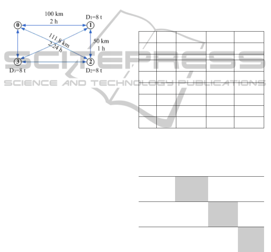
We consider the four node network of Figure 1,

with 3 different vehicles at node 0 to serve

customers 1, 2 and 3. We consider an average speed

of 50 km/h on each arc. Then the driving times t

between nodes are 1, 2 and 2.24 hours, depending on

the length of the arc. We assume a homogeneous

load demanded by each node as D

=8 ton. Service

times are set to s

=1 hour in all nodes by all

vehicles, and there are no toll costs.

Figure 1: Four-node example.

Table 1 shows the parameters associated to each

vehicle of the fleet. Table 2 shows the parameters

associated to fuel unit costs, external unit costs and

emission factors of vehicle types used.

As mentioned above, 12 instances are modelled

using the MILP problem. In case (b) we consider a

backhaul in node 2 with a demand of D

=-8 ton. In

case (c) we also assume a maximum driving time for

each vehicle of 8 h. And finally in case (d) we also

set a time window in node 1 of [3h, 5h].

We have used CPLEX 11.1 with its default

settings to solve the 12 MILP instances. Eight

different solutions have been found (Table 3).

The solutions associated to each instance and the

objective functions are illustrated in Table 4.

Table 1: Fleet parameters.

Vehicles (k) 1 2 3

(tons) 9.5 18 9.5

(€/h) 19.89 21.40 19.89

Type of fuel (r) Diesel Diesel Diesel

(l/100km) 17.50 19.80 17.50

feu

(l/ton·100km)

1.05 0.75 1.05

(€/day) 42.65 54.60 42.65

(€/km) 0.0590 0.0787 0.0590

Technology (t)

Rigid;

12-14_t;

Euro_IV

t=2

Rigid;

20-26_t;

Euro_IV

t=3

Rigid;

12-14_t;

Euro_II

t=1

Table 2: Unit costs.

DIESEL

(2010€/l) 0.9009

CO2

(2010€/ton) 25

CO2,DIESEL

(kg/l) 2.67

Pollutant (p) NOx NMVOC PM

(2010€/ton) 3439.8 529.2 76337.1

(gr/km) 5.50 0.207 0.1040

(gr/km) 2.65 0.008 0.0161

(gr/km) 3.83 0.010 0.0239

ne (2010€/ton-km) 0.00648

ae (2010€/ton-km) 0.00635

Table 3: Different optimal solutions.

Sol. Veh.

Optimal

Route

Load (ton)

Arrival

Time (h.)

0-3-0

0-2-1-0

8-0

16-8-0

7.24

#2 2 0-3-1-2-0 16-8-0-8 9.48

0-3-0

0-1-2-0

8-0

8-0-8

7.24

0-1-0

0-3-2-0

8-0

8-0-8

7.24

0-3-0

0-1-2-0

8-0

16-8-0

7.24

0-1-2-0

0-3-0

8-0-8

8-0

7.24

0-1-0

0-3-2-0

8-0

8-0-8

7.24

0-3-2-0

0-1-0

8-0-8

8-0

7.24

Table 4: Solutions and values of the three objective

functions for all the instances.

Inst. Sol.

O.F. 1 Total

Distances

O. F. 2

Total

Internal

Costs

O. F. 2

Total

Costs

1a #1

361,8 † 419,5 463,9

1b #2 323,6 † 358,3 † 402,0 †

1c #3

361,8 † 387,2 † 428,1

1d #4

461,8 † 498,6 538,6

2a #5 361,8 †

418,2 † 460,0 †

2b #2 323,6 † 358,3 † 402,0 †

2c #6 361,8 †

387,2 † 425,2 †

2d #7 461,8 †

468,6 † 511,6

3a #5 361,8 † 418,2 †

460,0 †

3b #2 323,6 † 358,3 † 402,0 †

3c #6 361,8 † 387,2 †

425,2 †

3d #8 461,8 † 468,6 †

510,5 †

† Optimal solution with that Objective Function

6 ANALYSIS OF RESULTS

Some implications of the results presented in Table

4 are as follows.

EVALUATING VEHICLE ROUTING PROBLEMS WITH SUSTAINABILITY COSTS

179

Optimal solutions which consider the traditional

objective function of minimizing total distance

travelled (Sol#1 to Sol#4) are not optimal in some

cases when the objective function includes costs’

parameters. But optimal solutions which consider

internal and external costs in the objective function

(Sol#5, #2, #6 and #8) are also optimal minimizing

distances or internal costs. The reason is that

minimizing internal costs is quite similar to

minimizing distances.

When a heterogeneous fleet is considered,

adding external costs implies the selection of the less

pollutant vehicles or the assignment of longer routes

to those vehicles (Sol#7 vs. Sol#8), maintaining

minimum total internal costs.

Depending on the type of VRP, the analysis of

performance measures must be different. Solutions

including backhauls reduce all the costs (see Table

4, Inst.b vs. Inst.a). But adding time constraints

increase the costs (see Table 4, Inst.d or Ins.c vs.

Inst.b). Using the total costs allows comparing

different solutions and selecting the most

appropriate. For example, Sol#8 is better than Sol#7

for the external cost, and also Sol#7 is better than

Sol#4 for the internal and external costs.

7 CONCLUSIONS

In this paper, a new mixed-integer linear

programming model for the Vehicle Routing

Problem with some realistic assumptions

(Heterogeneous Fleet, Time Windows and

Backhauls) is presented with a broader objective

function that accounts not just for the internal costs,

but also for external costs. With this model,

transportation companies can select the most

appropriate vehicles, determine the routes and

schedules to satisfy the demands of the customers,

reduce externalities and achieve a more sustainable

balance between economic, environmental and

social objectives.

An illustrative example with four nodes and

three different vehicles has been presented. 12

instances of the 4-node example have been solved

using three objective function and four variants. 8

different optimal solutions have been obtained and

they have been compared. Solution with the lowest

values of the total costs is the dominant solution and

must be selected.

Further research leads to the application of the

model to realistic numbers of customers. In larger

instances the development of heuristic algorithms

such as tabu search methods are needed.

ACKNOWLEDGEMENTS

This research has been fully funded by the Spanish

Ministry of Science and FEDER through grants

DPI2008-04788 and by the Andalusia Government

through grants P10-TEP-6332.

REFERENCES

Bektas, T. & Laporte, G. 2011. The Pollution-Routing

Problem. Transportation Research Part B,

doi:10.1016/j.trb.2011.02.004.

Bickel, P., Friedrich, R., Link, H., Stewart, L. & Nash, C.

2006. Introducing environmental externalities into

transport pricing: measurement and implications.

Transport Reviews, 26(4): 389–415.

Cordeau, J.-F., Laporte, G., Savelsbergh, M. W. P. &

Vigo, D. 2007. Vehicle routing. In: Barnhart, C.,

Laporte, G. (Eds.), Transportation, Handbooks in

Operations Research and Management Science, vol.

14: 367-428. Elsevier, Amsterdam, The Netherlands.

Dyckhoff, H., Lackes, R. & Reese, J. 2004. Supply Chain

Management and Reverse Logistics. Springer.

EMEP/EEA. 2010. Emission inventory guidebook 2009,

updated June 2010. European Environment Agency.

INFRAS/IWW. 2004. External costs of transport: update

study, INFRAS, Zurich.

INFRAS, CE Delft, ISI & University of Gdansk. 2008.

Handbook on estimation of external cost in the

transport sector. Produced within the study:

Internalisation Measures and Policies for All external

Cost of Transport (IMPACT), Delft, CE.

Maden, W., Eglese, R. W. & Black, D. 2010. Vehicle

routing and scheduling with time varying data: a case

study. Journal of the Operational Research Society,

61(3), 515–522.

Salhi, S. & Rand, G. K. 1993. Incorporating vehicle

routing into the vehicle fleet composition problem.

European Journal of Operational Research,

66:313_330.

Sniezek, J. & Bodin L. 2002. Cost Models for Vehicle

Routing Problems. Proceedings of the 35th Hawaii

International Conference on System Sciences, 1403-

1414.

Solomon, M. M. 1987. Algorithms for the vehicle routing

and scheduling problems with time window

constraints. Operations Research, 35(2):254_265.

Toth, P. & Vigo, D. 2002. The vehicle routing problem.

SIAM Monographs on Discrete Mathematics and

Applications, SIAM, 195–224.

ICORES 2012 - 1st International Conference on Operations Research and Enterprise Systems

180