MEANINGFUL THICKNESS DETECTION ON POLYGONAL
CURVE
Bertrand Kerautret
1,2
, Jacques-Olivier Lachaud
2
and Mouhammad Said
3
1
LORIA (UMR CNRS 7503), Nancy University, Nancy, France
2
LAMA (UMR CNRS 5127), University of Savoie, Le Bourget-du-Lac, France
3
LIRIS (UMR CNRS 5205), University of Lyon 2, Lyon, France
Keywords:
Shape analysis, Noise detection, Meaningful scale, Contour representation.
Abstract:
The notion of meaningful scale was recently introduced to detect the amount of noise present along a digital
contour. It relies on the asymptotic properties of the maximal digital straight segment primitive. Even though
very useful, the method is restricted to digital contour data and is not able to process other types of geometric
data like disconnected set of points. In this work, we propose a solution to overcome this limitation. It exploits
another primitive called the Blurred Segment which controls the straight segment recognition precision of
disconnected sets of points. The resulting noise detection provides precise results and is also simpler to
implement. A first application of contour smoothing demonstrates the efficiency of the proposed method. The
algorithms can also be tested online.
1 INTRODUCTION
Detecting if a contour is sampled at a meaningful
scale and estimate what are the correct scales to an-
alyze it (if they exist) is an important issue in shape
analysis. For instance, it makes easier the automated
parameterization in geometric shape analysis, contour
representation or pattern recognition. In general, the
noise is taken into account by a supervised parameter
chosen according to the input data quality. The choice
of the parameter is largely influential on the quality of
the process. For instance in a deformable boundary
segmentation technique, the smoothing parameter has
a great impact on the result.
Following a principle of perception from the
Gestalt theory, Desolneux et al. propose to detect
the meaningful edges of a grey level image by using
false alarm probability defined on the iso contours of
the image (Desolneux et al., 2001). This detection is
based on the image gradient and is not directly de-
fined for discrete contour representations. Along the
same lines, Cao introduces the notion of meaningful
good continuation (Cao, 2003) which relies on geo-
metric properties of the given curve. The false alarm
probability was simply approximated by a curvature
estimation of the input curve. Other applications of
Gestalt theory can be found in a recent article (Desol-
neux, 2011).
s = 1
s = 2
s = 3
s = 5
σ = 0.5
σ = 0.5
σ = 0.5
σ = 0.5
(a) (b) s = 3 (c) s = 5
(e) (f) (g)
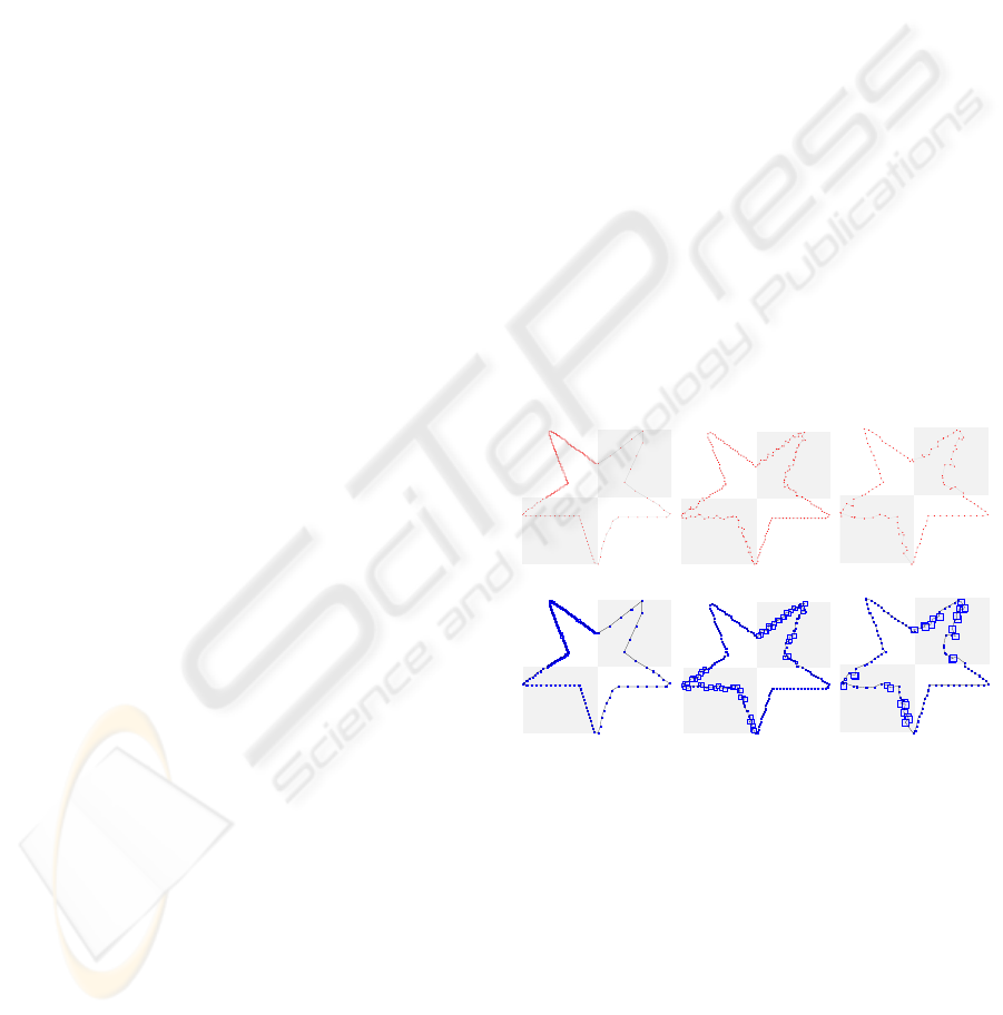
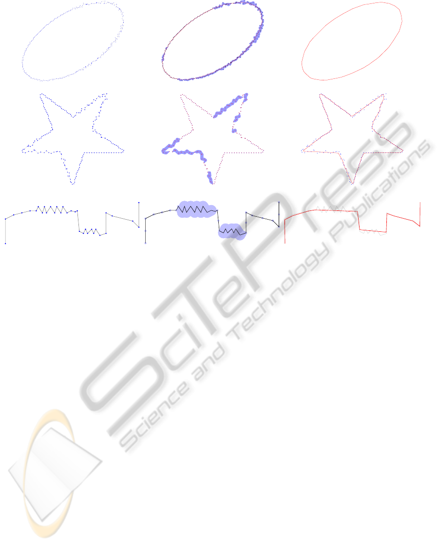
Figure 1: Noise detection on polygonal curves defined both
with different sampling rate (s), image (a) and with several
gaussian noise intensity (σ), images (b,c). The resulting
noise detection of polygons (a-c) is given on (e-f) where
the detected noise level is represented by boxes.
The concept of meaningful scale along digital
contour (i.e. boundary of a digital region) has been
introduced in a recent work to detect automatically
if the current scale is locally significant or not (Ker-
autret and Lachaud, 2009b). It relies on the study of
asymptotic properties of maximal digital straight seg-
ment which is a classic tool used to extract geomet-
ric parameter on a discrete contour (Lachaud et al.,
2005). More precisely the length of discrete maximal
372
Kerautret B., Lachaud J. and Said M. (2012).
MEANINGFUL THICKNESS DETECTION ON POLYGONAL CURVE.
In Proceedings of the 1st International Conference on Pattern Recognition Applications and Methods, pages 372-379
DOI: 10.5220/0003760903720379
Copyright
c
SciTePress

A
replacements
P
1
P
2
P
3
P
4
P
5
P
6
Q
1
Q
2
Q
3
Q
4
Q
5
Q
6
Q
7
Q
8
Q
9
Q
10
P
1
P
2
P
3
P
4
P
5
A
Length
L
1
0
Length
L
1
1
1
-thick BS
0
1
-thick BS
1
Q
1
Q
2
Q
3
Q
4
(a) (b)
Figure 2: Illustration of (a) a maximal DSS of characteristics (a,b,µ) = (2,5,0), and (b) two α-thick Blurred Segments with
α = 1 (denoted as 1-thick BS
i
with i = 0,1).
segment is analyzed on the contour represented at dif-
ferent scales to determine locally if a point is mean-
ingful or not. In opposition with the work of Cao, the
method can also detect what is the local best scale to
analyze the considered shape (if it exists).
The limitation of the meaningful scale method
lies mainly in the fact that the analysis is only pos-
sible on a sequence of simple 4 or 8-connected points
and cannot be applied on a general polygon such the
ones illustrated on Fig. 1. This restriction is due to
the intrinsic properties of the discrete primitive. In
this work, we introduce the new notion of meaning-
ful thickness by using a less restrictive primitive (the
α-thick Blurred Segment) that is described in the next
section.
2 MAXIMAL DIGITAL AND
BLURRED STRAIGHT
SEGMENT
Introduced in the 1970’s, the digital straightness has
been an active topic studied through many years, see
for instance (Rosenfeld, 1974; Dorst and Smeulders,
1984; Bruckstein, 1991), and (Klette and Rosenfeld,
2004) for a recent review. Its potential applications
are numerous from the definition of geometric estima-
tors like tangent, curvature (Kerautret and Lachaud,
2009a) to for instance polygonal contour representa-
tion (Bhowmick and Bhattacharya, 2007). Although
there are different definitions, we recall the classic
standard digital straight line (DSL) primitive used in
the concept of the meaningful scale detection.
A standard Digital Straight Line (DSL) is some
set {(x, y) ∈ Z
2
,µ ≤ ax −by < µ + |a|+ |b|}, where
(a,b,µ) are also integers and gcd(a,b) = 1. It is well
known that a DSL is a 4-connected simple path in the
digital plane. A digital straight segment (DSS) is a
4-connected piece of DSL. The interpixel contour of
a simple digital shape is a 4-connected closed path
without self-intersections. Given such a 4-connected
path C, a maximal segment M is a subset of C that is
a DSS and which is no more a DSS when adding any
other point of C\M.
A recognition process of a DSS is illustrated on
Fig.2 (a) where a maximal segment is recognized by
adding step by step the sequence of points: P
1
, Q
1
,
P
2
, Q
2
, P
3
, Q
3
, P
4
, Q
4
, P
5
, Q
5
, Q
6
, Q
7
, Q
8
, Q
9
. After
adding the point P
5
the DSS can only be extended on
the back (points Q
i
) since the point P
6
does not belong
to the segment. The discrete length of this DDS is
defined as the number of step and is denoted as L
j
where j is DSS number covering an initial point (L
0
=
14 in the example of Fig.2).
HW
VW
Figure 3: Illustration of the convex hull and its vertical and
horizontal thickness.
Blurred segments were introduced to address
noisy data (Debled-Rennesson et al., 2006). We use
the following definition (Faure et al., 2009): a set of
points is an α-thick Blurred Segment if and only if
its convex hull has an isothetic thickness less than a
given real number α. The isothetic thickness of a con-
vex hull is the smallest value between its vertical and
its horizontal width (denoted respectively as HW and
VW on Fig.3). In the same way as previously a maxi-
mal α-thick Blurred Segment can be defined as a seg-
ment which can not be extended to the front or to the
back.
An illustration is given on Fig.2 (b). An α-thick
Blurred Segment with α = 1 is recognized from the
point A by adding alternatively the points P
1
, Q
1
, P
2
,
MEANINGFUL THICKNESS DETECTION ON POLYGONAL CURVE
373

Q
2
and P
3
(denoted as 1-thickBS
1
). Neither the points
P
4
nor Q
3
can be added to the maximal 1-thickBS
1
since the resulting isothetic thickness will be greater
than α = 1. Another maximal segment 1-thickBS
0
covering the point A is illustrated in light color on
Fig. 2 (b). For each segment 1-thickBS
i
, its length L
1
i
is illustrated in light gray and constitutes an essential
property which will be exploited in the definition of
meaningful thickness introduced in the next section.
3 MEANINGFUL THICKNESS
DETECTION WITH MAXIMAL
BLURRED SEGMENT
Before introducing the new concept of Meaningful
Thickness we recall briefly the main idea of the mean-
ingful scale detection (Kerautret and Lachaud, 2009b)
and show the main inconvenient.
3.1 Asymptotic Property of Maximal
Segments
The meaningful scale detection relies on the analy-
sis of asymptotic property of maximal straight seg-
ments. This property is the discrete length (L
h
j
) of a
maximal segment belonging to a contour point given
at a digitization grid size h. In the following, we
will denote by Dig
h
(S) the Gauss digitization pro-
cess (Dig
h
(S) = X ∩hZ ×hZ). From different analy-
sis shown in (Lachaud, 2006; Kerautret and Lachaud,
2009b), several properties can be summed up as fol-
lows:
Property 1. Let S be a simply connected shape in R
2
with a piecewise C
3
boundary. Let P be a point of the
boundary ∂S of S. Consider now an open connected
neighborhood U of P on ∂S. Let (L
h
j
) be the digital
lengths of the maximal segments along the boundary
of Dig
h
(S) and which cover P. Then, the asymptotic
behaviour of the digital lengths follows these bounds:
if U is strictly convex or concave, then
Ω(1/h
1/3
) ≤ L
h
j
≤ O(1/h
1/2
) (1)
if U has null curvature, then
Ω(1/h) ≤ L
h
j
≤ O(1/h) (2)
The strategy to exploit this property was to trans-
form the initial discrete contour with several grid sizes
h while keeping the point associations and checking
the discrete contour consistency. The resulting analy-
sis shows precise and fine noise detection but is how-
ever not general for the analysis of other type of non
discrete contours.
A natural idea to generalize the analysis to polyg-
onal contour is to consider the primitive of the α-
thick Blurred Segment described in the previous sec-
tion which allows to deal with non integer points and
not necessary connected. The primitive presents an-
other advantage with its thickness parameter α that
can be used as a scale parameter.
3.2 Thickness Asymptotic Properties of
Blurred Segments
To define the notion of Meaningful Thickness with
the α-thick Blurred Segment, we need first to focus
on the asymptotic properties of the blurred segments
in the multi-thickness decomposition of a given con-
tour. The Euclidean length L will replace the digital
length L used in the previous Property1. L is defined
as the length of the bounding box obtained from the
α-thick Blurred Segment convex hull. Fig.2 (b) il-
lustrates such a bounding box with the length of two
1-thick Blurred Segments covering the point A (1-
thickBS
0
and 1-thickBS
1
). Their bounding boxes are
given respectively by the points P
1
,Q
1
,Q
2
,Q
3
,Q
4
and
Q
2
,P
2
,P
3
,P
1
,Q
1
.
When the Euclidean lengths of blurred segments
around a point of a polygonal contour is computed,
we observe an increasing sequence of lengths for
the increasing sequence of real thicknesses t
i
= ik
√
2
where k is the mean distance between consecutive
polygon vertices. When plotted in logscale, its slope
is related to the localization of the point in a flat or
curved zone. More precisely, letting (L
t
i
j
)
j=1,...,l
i
be
the Euclidean lengths of the blurred segments along
the digital contour and covering a point, we have ob-
served experimentally the following behavior:
Property 2. (Multi-thickness). The plots of the
lengths L
t
i
j
/t
i
in log-scale are approximately affine
with negative slopes as specified besides:
expected slope
plot curved part flat part
(log(t
i
),log(max
j
L
t
i
j
/t
i
)) ≈ −
1
2
≈ −1
(log(t
i
),log(min
j
L
t
i
j
/t
i
)) ≈ −
1
3
≈ −1
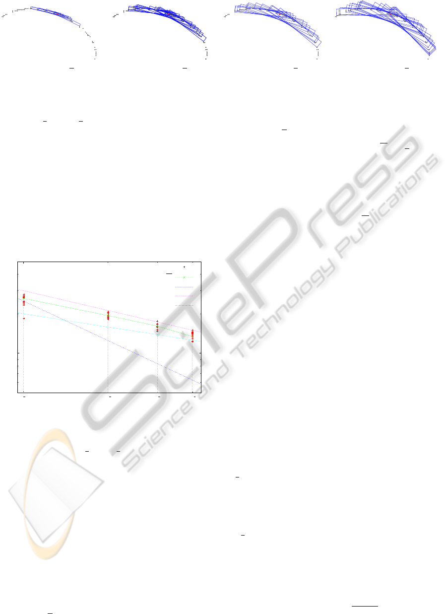
Fig.5 and Fig. 4 illustrates such a behaviour on
an ellipse shape represented by a disconnected set of
points with some missing parts. The set of α-thick
Blurred Segments covering a specific point P (l
i
seg-
ments cover P) is represented on Fig. 5 with four dif-
ferent thicknesses (t =
√
2, 2
√
2, 3
√
2, 4
√
2). For
each thickness t
i
, the lengths (L
t
i
j
)
j=1,..,l
i
are repre-
sented on the plot of Fig. 5. On this simple example
we can check that the segment length verifies the pre-
vious Property2 with their min and max values near
ICPRAM 2012 - International Conference on Pattern Recognition Applications and Methods
374
(a) t
1
=
√
2 (b) t
2
= 2
√
2 (c) t
3
= 3
√
2 (c) t
4
= 4
√
2
Figure 4: Covering a point of the initial contour by the blurred segments obtained with different thicknesses (t
i
). For each
thickness the blurred segments covering the considered point (drawn in red) are drawn with blue boxes.
the slope −
1
2
and −
1
3
which correspond to the hy-
pothesis of a curved contour part. Other measures on
different shapes are given in (Said, 2010).
As in the multi-scale computation (Kerautret and
Lachaud, 2009b), the multi-thickness results allows
us to distinguish between curved and flat parts of an
object boundary. This approach is not valid on points
that are (1) a transition between a curved and a flat
part, (2) corner points. Finally, this technique as-
sumes smooth objects with perfect digitization: if the
digital contour has been damaged by noise or digiti-
zation artefact, these characterizations do not hold.
Blurred Segment Length L
x
10
x**(-1.0)*25
x**(-1.0/2.0)*30
x**(-1.0/3.0)*20
α-thick Blurred Segment length L
x
j
α-thick Blurred Segment mean length
L
x
p
(2) 2
p
(2)
3
p
(2)
4
p
(2)
Thickness
Figure 5: Illustration of the Lengths
L
x
j
from the set of
α-thick Blurred Segments given from illustration of Fig. 4.
The lines of slope −1, −
1
2
and −
1
3
are also given to illus-
trate the reference constraint of Property2.
Although the two last remarks seem problematic
for analyzing shapes, we will use them to detect lo-
cally the amount of noise and to extract the local
meaningful thickness.
3.3 Local Geometric Evaluation with
Multi-thickness Criterion
We analyze now the local geometry of some point P
on a polygonal curve C having a mean distance be-
tween vertices equals to k. For various values of thick-
ness t
i
= ik
√
2, i = 1..n, we compute the Euclidean
lengths L
t
i
j
of the blurred segments of C. For a given
thickness ik
√
2, the average length of all blurred seg-
ments covering a point P is denoted as L
t
i
=
1
l
i
∑
j
L
t
i
j
,
where l
i
represents the number of blurred segments
containing P. Fig.4 illustrates the blurred segments
covering a point, obtained on the contour with several
values of thickness t
i
.
We define the multi-thickness profile P
n
(P) of a
point P as the graph (log(t
i
),log(L
t
i
/t
i
))
i=1,...,n
. We
also define the ideal multi-thickness criterion µ
n
(P)
of a point P on the boundary of a digital object as
the slope coefficient of the simple linear regression
of P
n
(P). Property 2 indicates that µ
n
(P) should be
around -1 if P is in flat zone, whereas it should be
within [−1/2, −1/3] if P is in a strictly convexor con-
cave zone.
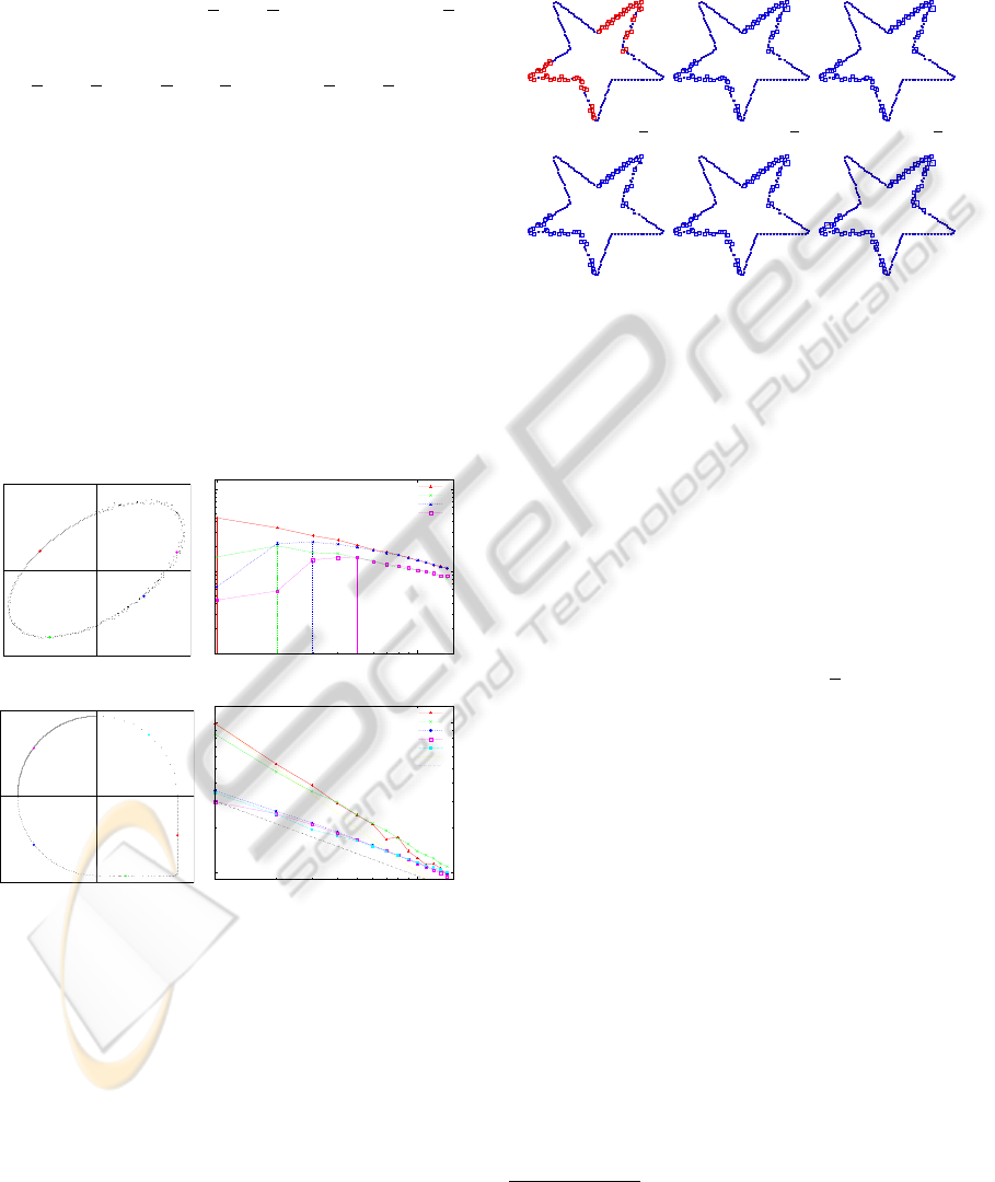
Detecting Noise and Local Meaningful Thickness.
The multi-thickness profile can be used to detect
noisy polygonal curves. We show on Fig.6 (b) the
multi-thickness profile of a point P
A
located on a per-
fectly digitized curved zone and the multi-thickness
profiles of the points P
B
, P
C
and P
D
located in noisy
zones (image (a)). On the first profile, the decreas-
ing affine relation is immediately visible. On the lat-
ter profiles, it is increasing at fine resolution and then
falls back on a decreasing affine profile after a given
thickness. We apply also the multi-thickness pro-
files on the polygonal curve with flat and curved ar-
eas (Fig. 6 (c,d)). The difference between them is the
slope of the affine relation of the profiles (slope near
−
1
2
for the plots of points P
C
, P
D
and P
E
and near −1
for the plots of points P
A
and P
B
).
We then introduce a noise threshold T
m
which
discriminates between a curved zone and a noisy
zone. This threshold should be somewhere between
] −
1
3
,0[. However after several experiments on noisy
shapes it appears that the use of the upper threshold
value T
m
=0 gives best results both on curved or flat
noisy parts.
A meaningful thickness of a multi-thickness pro-
file (X
i
,Y
i
)
1≤i≤n
is then a pair (i
1
,i
2
), 1 ≤i
1
< i
2
≤ n,
such that for all i, i
1
≤ i < i
2
,
Y
i+1
−Y
i
X
i+1
−X
i
≤ T
m
, and the
property is not true for i
1
−1 and i
2
. The first mean-
MEANINGFUL THICKNESS DETECTION ON POLYGONAL CURVE
375
ingful thickness (i
1
) of a point P can be considered
as a noise level and is denoted as t
τ
(P) = i
1
. Note
that this noise level definition does not depend of the
second value i
2
.
From the example of Fig. 6 (a,b), the point A lo-
cated on a smooth contour part, has a meaningful
thickness equals to (1
√
2,14
√
2) with t
τ
(A) = 1
√
2.
For the noisy contour parts, the points P
B
, P
C
and
P
D
have respectively a meaningful thickness equals to
(2
√
2,14
√
2), (3
√
2,14
√
2) and (5
√
2,14
√
2). This
example show that the meaningful thickness is well
identified and is related on the noise intensity. More-
over the other example of Fig.6 (c,d) demonstrates
that the meaningful thickness detection is not de-
graded by changes of the sampling rate. This experi-
ment will be also confirmed in the next section.
To improve the notion ideal multi-thickness crite-
ria on noisy data, we adapt it with the use the previous
meaningful thickness. Then, if (i
1
,i
2
) is a meaning-
ful thickness of some profile P
n
(P), the (i
1
,i
2
)-multi-
thickness criterion µ
i
1
,i
2
(P) of point P is then the slope
coefficient of the simple linear regression of P
n
(P) re-
stricted to its samples from i
1
to i
2
. This definition
will be used in experiments of the following section.
P
A
P
B
P
C
P
D
σ
1
= 0
σ
2
= 0.5
σ
3
= 1
σ
4
= 1.5
1
10
100
10
α
τ
(P
D
)
α
τ
(P
C
)
α
τ
(P
B
)α
τ
(P
A
)
Multi-thickness profile P
A
Multi-thickness profile P
B
Multi-thickness profile P
C
Multi-thickness profile P
D
(a) (b)
P
A
P
B
P
C
P
D
P
E
10
100
1 10
x**(-1.0)*100
x**(-1.0/2.0)*30
Multi-thickness profile P
A
Multi-thickness profile P
B
Multi-thickness profile P
C
Multi-thickness profile P
D
Multi-thickness profile P
E
(c) (d)
Figure 6: Multi-thickness profiles (b,d) obtained on two
sampled contours (a,c). The curve (a) was obtained by
adding gaussian noise with std deviation σ.
4 EXPERIMENT AND
COMPARISON
Before applying comparisons of the meaningful
thickness detection with the meaningful scale ap-
proach, it is important to measure the influence of
the parameter used in the method. The first param-
eter is the maximal thickness (t
max
) used to create the
meaningful thickness profile and the second one is the
minimal slope to consider a point as noise (parameter
T
m
).
(a) t
max
= 5
√
2 (b) t
max
= 10
√
2 (c)t
max
= 15
√
2
(d) T
m
= 0.2 (e) T
m
= 0.0 (f) T
m
= −0.2
Figure 7: Evaluation of the independence of the meaning-
ful thickness detection from the different parameters. The
size of the blue boxes represents for each point the obtained
meaningful scale or thickness α
τ
. The first row presents the
evaluation by varying the maximal thickness used to define
the multi-thickness profile (t
max
). The red color indicates
present on image (a) indicates that there exists no mean-
ingful thickness less than t
max
. The second row shows the
stability by the change of the noise threshold parameter T
m
.
The first experiment of Fig. 7 (a-c) shows that the
parameter t
max
does not change the quality of the de-
tection. The images (b,c) show quite similar noise
levels. For the first experiment (a) the pixels drawn
in red show that no meaningful thickness was found
since the maximal value t
max
= 5
√
2 was too small
and the meaningful thickness is in fact greater than
t
max
. The stability for the other parameter T
m
was also
experimented on Fig. 7 (d-f). The default value of T
m
set to 0 was experimented as giving best results but we
can see that a large change of this parameter does not
really change the noise detection quality. Other ex-
periments
1
confirm that the proposed method can be
considered as parameter free. Note that for all other
experiments these parameters were set to t
max
= 15
and T
m
= 0 (and also in the online demonstration).
4.1 Experiment of Meaningful
Thickness Detection
Comparison with the Meaningful Scale. To evalu-
ate the quality of the meaningful thickness detection
we perform some comparisons with the meaningful
scale detection. Fig.8 presents results on a digital
1
Other experiments can be done online (Kerautret et al.,
2011)
ICPRAM 2012 - International Conference on Pattern Recognition Applications and Methods
376
shape where noise was added manually to the initial
curve. The detection accuracy appears as precise as
the meaningful scales if we except some corners of
the polygon which tends to be detected as noise with
the method based on the meaningful thickness (see
close up view of image (e) and (f)). Note that the
meaningful scale detection appears to be a little more
dynamic than the meaningful thickness. From a com-
putational point of view, the meaningful scale method
is faster (76 ms and 87 ms for respectively(b) and (e))
than the meaningful thickness approach (542 ms and
485 ms. for respectively (c) and (f) on a Mac OS X 2.8
Ghz Core 2 Duo), but the thickness detection uses an
O(n
2
) version of the blurred segment detection while
all maximal straight segments are computed in linear
time according to the number of contour point. More
objective time comparisons are let to future works.
(a) 828 points (d) 966 points
(b) Meaningful scale
(Kerautret and Lachaud,
2009b)
(e) Meaningful scale
(Kerautret and Lachaud,
2009b)
.
(c) Meaningful thickness. (f) Meaningful thickness.
Figure 8: Comparison between meaningful scale (Kerautret
and Lachaud, 2009b) (second line) and meaningful thick-
ness (third line). The size of the blue boxes represents for
each pixel the obtained meaningful scale or thickness α
τ
.
The amount of noise is well evaluated everywhere.
Experiment on Polygonal Curves. The new possi-
bility to detect the meaningful thickness on polygo-
nal curves was experimented in Fig. 9. The first ex-
periment applies the detection on a non uniformly
sampled contour (contour of Fig. 6 (c)). The result-
(a) (b)
(c) (d)
(e) ε = 0.001 (f) ε = 10
(Cao, 2003) (Cao, 2003)
Figure 9: Meaningful thickness detection on polygonal
curves. The polygonal curve (a) was obtained after apply-
ing a sampling process defined for each quadrant (the same
than for Fig. 6 (a)). The polygon (b) was obtained after
adding some noise specifically to each sector and its de-
tected meaningful thickness is represented in (c). (d) shows
the same results obtained on the ellipse of the Fig.6 (a) and
(e,f) show comparisons with the meaningful good continu-
ation method (Cao, 2003) (in thick red plot) obtained with
different values of ε.
ing meaningful thickness is everywhere 1 as expected
(Fig.9 (a)). By adding noise on different quadrants
of the previous contour, the detector consistently in-
creases the meaningful thickness (image (c)). The
other experiment applied on ellipse also show nice
meaningful thickness detection (d).
To apply comparisons with other comparable ap-
proach, we have experimented the method of the
meaningful good continuation of Cao (Cao, 2003).
As briefly described in the introduction and contrary
to our method this approach has a parameter ε which
can be tuned to adjust the level of what can be con-
sidered as meaningful or not. On results presented
on Fig.9 (e,f) we can see that the meaningful contour
parts are well identified and are not in contradiction
with the meaningful thickness detection but our ap-
proach does not need to set any parameter and can
also give directly the meaningful thickness (if it ex-
its).
MEANINGFUL THICKNESS DETECTION ON POLYGONAL CURVE
377

(a) source (b) iso contours
(c) Meaningful contours (d) straight parts
Figure 10: Application to meaningful contours extraction
(image (c)) using all iso level contours (image (b)). The
straight parts obtained from meaningful multi-thickness
profile are represented in (d).
Application to Extract Meaningful Contours in
Images. The meaningful thickness detection can be
applied on every level set of the image. Fig.10 (b)
shows all the set of such a contour extracted after
tracking the frontier of the connected components de-
fined from each threshold step. Here 256 gray lev-
els were considered with a step of 10. The image
(c) of Fig. 10 show all the contour parts with a mean-
ingful thickness equals to one (i.e. no noise). From
all the contours, we also detect the straight contour
parts by applying a threshold to the slope of the multi-
thickness criterion µ
i
1
,i
2
(P) by −0.46.
4.2 Simple Application for Contour
Smoothing
This meaningful thickness detection can be used in
numerous applications (in particular, in most of the
algorithms which use the α-thick Blurred Segment
primitive). We present here a simple potential appli-
cation of contour smoothing by taking the meaningful
thickness as a constraint for a curve reconstruction.
The reconstruction method is an iterative process that
computes the new points as a weighted average of its
neighbors, constrained by the meaningful thickness
(displayed in light blue on Fig. 11 (b,e,h)). Note that
these constraints were defined from the meaningful
thickness on all non meaningful edges by using linear
interpolation between the vertex of the polygon.
The resulting reconstruction visible on images
Fig.11 (c,f,i) show very fine polygonal contours
where noise are no more visible. Moreover all ini-
tial contour parts with no noise are well preserved af-
ter the reconstruction. Another interesting quality is
visible with the preservation of all discontinuities in
particular for the open contour of Fig.11 (g-i).
5 CONCLUSIONS
A new concept of meaningful thickness was pre-
sented. The proposed method can be considered as
parameter free and can be applied both on discrete or
polygonalcontour. The results are very promising and
open the door to new unsupervised applications. The
simple contour smoothing application is a first appli-
cation which already shows fine results without the
need to set any particular parameter. The proposed
method is simple to implement and the user can test
the algorithm with their own data (Kerautret et al.,
2011). The source code is also already available from
the ImaGene library (Ima, 2011) and is planned to be
integrated as a module in the new DGtal library (DGt,
2011).
REFERENCES
(2011). DGtal: Digital geometry tools and algorithms li-
brary. http://liris.cnrs.fr/dgtal.
(2011). Imagene, Generic digital Image library. http://
gforge.liris.cnrs.frs/projects/imagene.
Bhowmick, P. and Bhattacharya, B. B. (2007). Fast
polygonal approximation of digital curves using re-
laxed straightness properties. IEEE Trans on PAMI,
29(9):1590–1602.
Bruckstein, A. (1991). Self-similarity properties of digi-
tized straight lines. Contemp. Math, 119:1–20.
Cao, F. (2003). Good continuations in digital image level
lines. In Proc. of ICCV 2003, volume 1, pages 440–
448. IEEE.
Debled-Rennesson, I., Feschet, F., and Rouyer-Degli, J.
(2006). Optimal blurred segments decomposition of
noisy shapes in linear time. Computers & Graphics,
30(1).
ICPRAM 2012 - International Conference on Pattern Recognition Applications and Methods
378
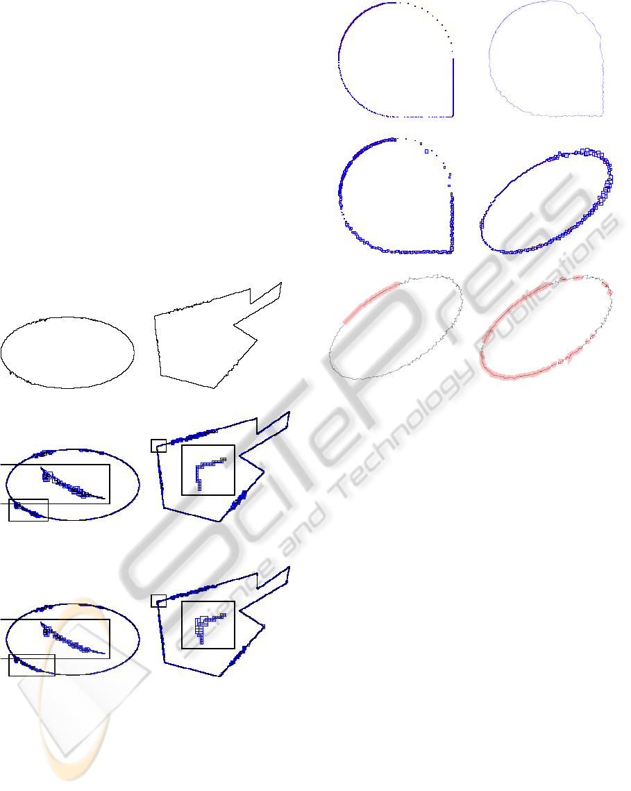
source contour meaningful thickness constraint resulting reconstruction
(a) (b) (c)
(d) (e) (f)
(g) (h) (i)
Figure 11: Application of contour smoothing using the meaningful thickness on several shapes. The initial noisy source
contour are given in image (a,d,g). The blue areas represent the noise constraints (b,e,h) and the resulting smoothed contour
is represented in red on (c,f,i).
Desolneux, A. (2011). A probabilistic grouping principle to
go from pixels to visual structures. In Proc of DGCI,
volume 6607 of LNCS, pages 1–13. springer.
Desolneux, A., Moisan, L., and Morel, J.-M. (2001). Edge
detection by helmholtz principle. Journal of Mathe-
matical Imaging and Vision, 14:271–284.
Dorst, L. and Smeulders, A. (1984). Discrete representation
of straight line. IEEE Trans. Patt. Anal. Mach. Intell,
6:450–463.
Faure, A., Buzer, L., and Feschet, F. (2009). Tangential
cover for thick digital curves. Pattern Recognition,
42(10):2279 – 2287.
Kerautret, B. and Lachaud, J.-O. (2009a). Curvature
estimation along noisy digital contours by approx-
imate global optimization. Pattern Recognition,
42(10):2265 – 2278.
Kerautret, B. and Lachaud, J.-O. (2009b). Multi-scale anal-
ysis of discrete contours for unsupervised noise detec-
tion. In Proc. IWCIA, volume 5852 of LNCS, pages
187–200. Springer.
Kerautret, B., Lachaud, J.-O., and Said, M. (2011). Mean-
ingful thickness detection demonstration. http://
kerrecherche.iutsd.uhp-nancy.fr/MeaningfulThickness.
Klette, R. and Rosenfeld, A. (2004). Digital straightness–a
review. Discrete Applied Mathematics, 139(1-3):197
– 230.
Lachaud, J.-O. (2006). Espaces non-euclidiens et analyse
d’image : mod`eles d´eformables riemanniens et dis-
crets, topologie et g´eom´etrie discr`ete. Habilitation
`a diriger des recherches, Universit´e Bordeaux 1, Tal-
ence, France. (en franc¸ais).
Lachaud, J.-O., Vialard, A., and de Vieilleville, F. (2005).
Analysis and comparative evaluation of discrete tan-
gent estimators. In Proc. DGCI, volume 3429 of
LNCS, pages 140–251. Springer.
Rosenfeld, A. (1974). Digital straight line segments. IEEE
Trans. Comput., 23:1264–1269.
Said, M. (2010). G´eom´etrie multi-r´esolution des objets dis-
crets bruit´es. PhD thesis, University of Savoie.
MEANINGFUL THICKNESS DETECTION ON POLYGONAL CURVE
379
