CONTINUOUS-TIME REVENUE MANAGEMENT IN CARPARKS

A. Papayiannis

, P. Johnson

, D. Yumashev

, S. Howell

, N. Proudlove

and P. Duck

School of Mathematics, University of Manchester, Oxford Road, M13 9PL, Manchester, U.K.

Manchester Business School, University of Manchester, Manchester, U.K.

Keywords:

Expected revenue, Rejection policy.

Abstract:

In this paper, we study optimal revenue management applied to carparks, with primary objective to maximize

revenues under a continuous-time framework. We develop a stochastic discrete-time model and propose a

rejection algorithm that makes optimal decisions (accept/reject) according to the future expected revenues

generated and on the opportunity cost that arises before each sale. For this aspect of the problem, a Monte

Carlo approach is used to derive optimal rejection policies. We then extend this approach to show that there

exists an equivalent continuous-time methodology that yields to a partial differential equation (PDE). The

nature of the PDE, as opposed to the Monte Carlo approach, generates the rejection policies quicker and causes

the optimal surfaces to be signiﬁcantly smoother. However, because the solution to the PDE is considered not

to solve the ‘full’ problem, we propose an approach to generate optimal revenues using the discrete-time

model by exploiting the information coming from the PDE. We give a worked example of how to generate

near-optimal revenues with an order of magnitude decrease in computation speed.

1 INTRODUCTION

Over the last twenty years, cars have formed the main

transportation system for people worldwide, espe-

cially in developed countries. Since parking is essen-

tial for cars, this creates an opportunity for carparking

owners to exploit the increased demand to maximize

their turnover. This can be achieved through revenue

management (RM) techniques, such as those used in

the hotel industry, where customers purchase multiple

units in one transaction. Nevertheless, in carparking,

most research has focused upon the problem of re-

ducing trafﬁc congestion; For example, (Young et al.,

1991) argue that carparks play a major role in the

planning and management of transportation systems

and thus, appropriate parking pricing polices can be

used to reduce trafﬁc congestion. A sample list of re-

lated work includes (Vickrey, 1969), (Vikrey, 1994),

(Young et al., 1991), (Verhoef et al., 1995), (Teodor-

ovi´c and Vukadinovi´c, 1998), (Arnott and Rowse,

1999) and (Zhao et al., 2010). Whilst the literature

upon carparking RM is small, there are two wor-

thy studies of mention. The ﬁrst is (Teodorovi´c and

Luˇci´c, 2006), who propose an “intelligent” parking

space inventory control system, based on fuzzy logic

and integer programming techniques. They study the

problem of maximizing revenues when customer ar-

rival and departure times are stochastic, assuming dif-

ferent parking tariffs (prices). For a parking request

of a particular tariff, it is possible to know the per-

centage of the capacity remaining and the relative re-

quests’ revenue, as well as the percentage of all future

requests that make less relative revenue than the cur-

rent request; in this way, fuzzy rules are generated

(for detailed information in creating fuzzy rules, the

reader is referred to the work of (Wang and Mendel,

1992)). The problem is studied under several scenar-

ios and the results show that the relative error (be-

tween the proposed algorithm and the optimal upper

bound) never exceeds 10%. The initial setup of their

objective function has strong similarities to the setup

of our discrete-time model; however, their algorithm

is assumed to be able to “recognize” the type of the

request and to direct it to the appropriate fuzzy rule

base, in which a decision is made. Our system com-

bines all booking requests from both customers sets

in consideration, so that it makes a decision to ac-

cept/reject a request without knowing the booking set

each request comes from.

(Onieva et al., 2011) also study revenue manage-

ment being applied in carparks. They consider the

presence of a group of subscribers along with the

individual customers while the arrivals are assumed

to follow a non-homogeneous Poisson distribution.

They examine the problem under both a deterministic

and a stochastic environment and they develop three

Papayiannis A., Johnson P., Yumashev D., Howell S., Proudlove N. and Duck P..

CONTINUOUS-TIME REVENUE MANAGEMENT IN CARPARKS.

DOI: 10.5220/0003762800730082

In Proceedings of the 1st International Conference on Operations Research and Enterprise Systems (ICORES-2012), pages 73-82

ISBN: 978-989-8425-97-3

 2012 SCITEPRESS (Science and Technology Publications, Lda.)

different algorithms for capacity allocation; a ﬁrst-

come-ﬁrst-served, distinct and nested method. Us-

ing these simulation techniques, proﬁt maximization

were investigated, although little insight into the core

dynamics of the model was supplied. Their results

suggest that a stochastic model using nested alloca-

tion provides revenues that are closest to the optimal

values.

Within this study we assume the following:

1. Their is a ﬁnite ﬁxed number of spaces in a

carpark. Fixed capacity means that no more rev-

enue can be generated when there are no spaces

left.

2. The inventory is perishable and it can be sold in

advance or on arrival.

3. The demand for the product is time-invariant.

The main objective of our study is to Maximize

Proﬁts by Optimally Managing the Bookings in a

Continuous-Time Environment. What makes it dis-

tinct in our carparkingrevenue maximization problem

is the assumption of a continuous time framework.

We consider a carpark operating under the above

conditions and a target time T for which the spaces

must be used; for this two approaches are introduced.

We begin by generating sets of bookings using a Pois-

son distribution. The bookings arrive continuously,

but the cars are assumed to occupy the parking slots

for discrete periods of time, ∆t. The bookings are

allocated a price rate per day according to their du-

ration of stay (the more the stay days, the less the

price paid per day). We develop a discrete-time model

that makes a decision (accept/reject) for each one, in

the order the bookings are recorded. The decision

is based on the expected revenues generated in the

carpark and on the opportunity cost that arises before

each sale. In particular, we develop a rejection al-

gorithm according to which, given there is capacity

available, we do not sell any space for time T at any

time prior,t < T, for less money than what we expect

to receive for it in the future.

Then, a continuous-time model is introduced,

leading to a partial differential equation (PDE); The

methodology behind the derivation lies in the work of

(Gallego and van Ryzin, 1994) who proposed a deci-

sion tree approach. The PDE approach aims to repli-

cate the results of the discrete-time model when ∆t

tends to zero. The continuous model is based on the

probability distributions used previously to generate

the bookings. Instead of looking at the revenues gen-

erated within a ﬁnite time period, the model calculates

the rate at which the value of the carpark changes dur-

ing an instant of time. Again, bookings are allowed

to request any length of stay, but the rejection policy

will make a decision at each time period individually;

given a number of periods requested by a booking, the

policy may deny a parking slot for some of these peri-

ods, but still collect the revenues from the periods that

are accepted. Thus, the PDE is assumed not to solve

the ‘full’ problem.

Each approach will generate an optimal rejection

policy, based on which the revenues will be maxi-

mized. The slight difference in the manner in which

the rejection algorithms work, will generate slightly

higher revenues for the PDE

. However, the use of the

PDE is favourable as it produces much quicker and

smoother results. Therefore, we examine the case of

using the rejection algorithm in the Monte Carlo ap-

proach but with the opportunity costs (rejection pol-

icy) being calculated from the PDE. We show under

which conditions, the use of the PDE rejection pol-

icy generates maximum revenues for the full problem

and, in the case of near optimal revenues, we explain

the adjustments that have to be implemented.

The remainder of this report is organized as fol-

lows. In section 2, we deﬁne the problem, list the

set of assumptions used and develop the discrete-time

model. The continuous-time PDE model is intro-

duced and derived in section 3 with the numerical

results from both approaches to follow in section 4.

Section 5 presents our conclusions and thoughts for

future research in this area.

2 PROBLEM FORMULATION

2.1 The Model

We begin by describing the structure of the book-

ings. Each booking consists of three characteristics,

the time the booking is made, the time of arrival to the

carpark and the time of departure from the carpark.

Therefore, each booking i can be written as a vector,

namely





= t

+ η

= t

+ ξ





(1)

where t

denotes the booking time, t

the arrival time

with η denoting the pre-booking time and t

the de-

parture time with ξ denoting the duration of stay.

Bookings arrive in a continuous time; each one

requires a space in the carpark for a particular time

period and, thus, the customer is required to pay an

amount of money according to his/her duration of

stay.

To achieve this, any given time intervalt ∈ [a,b] is

Justiﬁcation on this is shown in section 4.

ICORES 2012 - 1st International Conference on Operations Research and Enterprise Systems

split into K discrete time steps, each of length ∆t, so

that

= a+ k∆t. for k = 0, 1,...,K.

Then, if C

denotes the number of cars present in

the car park at any time during the period t ∈ [t

k+1

we have

∑

f(B

,k)

where

f(B, k) =











1 if t

≤ t

< t

k+1

1 if t

< t

≤ t

k+1

1 if t

< t

and t

> t

k+1

0 otherwise

(2)

Note that we discount cars departing at t = t

k+1

being present during the period.

The duration of stay for a booking is, then, the number

of periods at which this booking is present in the car

park,

∑

f(B

,k). (3)

Now, suppose that the price rate per day (period) for a

booking B

changes according to a log-linear

pricing

function of the form

Ψ(ξ

) = ψ

+ ψ

−µξ

(4)

where ξ is the duration of the i

booking in days (pe-

riods) and ψ

, ψ

are positive constants and µ is the

decaying coefﬁcient.

Therefore, the revenue generated in the k

period

over all bookings is

∑

f(B

,k)Ψ(ξ

) (5)

and the total revenue R for the carpark is

∑

f(B

,k)Ψ(ξ

). (6)

2.2 Generating Bookings

The bookings are generated using a Poisson distribu-

tion with constant intensity λ

. Thus, λ

indicates

the average number of bookings made during a day

(the standard unit of analysis in this paper). Even

though we assumed that the average number of book-

ings made in a day is known, this is a stochastic prob-

lem because their exact number is still unknown.

Our intuition indicates that a pricing function of this

form is more common to be used in a real carpark, and it

is easy to work with. A log-linear pricing function requires

that the price rate per day (period) decreases monotonically

in the number of days requested but, at the same time, it

guarantees that the daily price never drops below a lower

minimum we choose.

The time of the next booking can be calculated as

follows

= t

n−1

−

log(u

), (7)

where u

is a random variable from the uniform dis-

tribution and t

n−1

the time of the last booking. If we

know that the average time between booking and ar-

rival is

η units of time and the average time between

arrival and departure is

ξ units of time, then we can

use Poisson processes with intensities λ

= 1/

η and

= 1/

ξ to model the arrival and duration of stays,

respectively. Therefore, by knowing the last booking

we can generate the next booking as:

i+1





= t

− (1/λ

)log(u

)

= t

− (1/λ

)log(u

n+1

)

= t

− (1/λ

)log(u

n+2

)





. (8)

2.2.1 Notation and Further Assumptions

(i) No discounting takes place, for simplicity. We

do not consider the time-value of money as the

report’s objective is to examine the performance

of the rejection algorithm.

(ii) There is no marginal cost incurred after a sale.

This is valid, because one can always express

price as the increment above cost. Thus, the ex-

pressions “revenue” and “proﬁt” will be used in-

terchangeably.

(iii) There are no cancellations; if a booking for a

particular duration is accepted, then the cus-

tomer will show up and pay with probability al-

most surely.

(iv) Two types of customers are considered - be-

cause there is no time variation, demand inten-

sities can be set to ﬁxed values for the entire

time horizon. Each set of parameters is care-

fully chosen to distinguish between the different

customers types:

• Low-paying customers

Leis

∼







= 5

= 1/14

= 1/7

(9)

These customers book early in advance to

take advantage of any discounts or promo-

tions, they require a space for long periods

and usually these represent leisure customers.

• High-paying customers

Busi

∼







= 25

= 1/3

= 1

(10)

CONTINUOUS-TIME REVENUE MANAGEMENT IN CARPARKS

These customers book just before or on

arrival. High-paying customers are usu-

ally business customers who are not ﬂexible

within dates, and thus they are willing to pay

full prices for just a short period of time.

These two sets of customers are combined ac-

cording to the time the bookings are made, so

that the system makes a decision about bookings

in the order they arrive and do not know which

booking set they come from.

2.2.2 Rejection Policy and Expected Values

The manager of the carpark can reject a request for

a space if they so choose. If the booking is rejected

then the customer cannot change their length of stay

to be accepted, the potential revenue for each period

of stay is lost. As such the bookings will be called

group bookings over different days and hence differ-

ent products. All decisions must be based on current

information and without knowledge of future events,

making it a non-anticipating policy. We call a pol-

icy that satisﬁes this criteria an admissible policy, de-

noted by π.

Thus, letV(C,Q,t;k) to denote the expected value

of the carpark of total capacity C with Q spaces re-

maining at time t until the space is used at time period

. By equation (5), this is

V(C,Q,t;k) = E

∑

i=i

∗

f(B

,k)Ψ(ξ

)

where i

∗

indicates the next booking made after t.

Since the goal is to maximize expected revenues, we

can write the problem as,

Maximize:

V(C,Q,t;k) = max

(

∑

i=i

∗

f(B

,k)Ψ(ξ

)

(11)

subject to:

0 ≤ C

≤ C, ∀k = 0,1,...,K, (12)

where π ∈ Π is any policy from the set of all admissi-

ble rejection policies. The capacity constraint in (12)

requires that the number of cars present in any period

should never exceed the total capacity of the carpark.

The quantityV(C, Q,t;k)−V(C,Q−1,t;k), is the

opportunity cost lost, incurred when we move from a

carpark of total capacity C with Q spaces remaining

at time t to one with Q− 1 spaces left. This quantity

suggests how much the q

unit of space is expected

to be worth at time t, denoted as the Expected Added

Value of the space at time t.

2.3 Rejection Algorithm

Our rejection algorithm is based on (Gallego and van

Ryzin, 1994) and Littlewood’s Rule ((Littlewood,

1972)), and suggests that a booking (at t

) will be

rejected if the total revenue generated is lower than

the expected revenue of all potential future bookings

that the car will displace over all periods it is present

in the carpark. In other words, it makes sense to

accept the booking i, only if the price satisﬁes:

Ψ(ξ

) > V(C,Q,t

;k) −V(C, Q− 1,t

;k) (13)

However, the booking decision should be taken ac-

cording to the total length of stay and not for each

day period individually; so for the ith booking made

within the period t

we ﬁnd it convenient to introduce

the Added Value across all periods during which the

car is present to be:

A =

∑

f(B

,k)[Ψ(ξ

)−

(V(C,Q,t

;k) −V(C, Q− 1,t

;k))], (14)

with n ≤ k. Then, the rule is

Accept if: A ≥ 0

Reject if: A < 0.

That demand is time invariant along with the no

discounting assumption enable us to calculate the ex-

pected value V going backward and forwards in time

at the same time. Therefore, the expected value of the

carpark of total capacity C with Q

spaces remaining

at t

for the space to be used at t

V(C,Q

;k) = V(Q

,0;k− n) = v

k−n, j

The resulting 2D-matrix v will then be used to deter-

mine the rejection policy π in the following algorithm;

2.3.1 Optimal Rejection Policy Algorithm

1. Choose a booking horizon T with K periods suf-

ﬁciently large to capture nearly all of bookings in

each set and a maximum capacity for the carpark

2. Initialize the rejection matrix v

= 0 so the value

of a space is zero, where v

is the qth guess at the

solution of the rejection algorithm v.

3. Use Monte-Carlo to generate booking sets in

within the time interval [0,T].

4. Evaluate the expected value of the carpark (of to-

tal capacity C) at time t for all time periods t

and

ICORES 2012 - 1st International Conference on Operations Research and Enterprise Systems

Table 1: Parameters Used.

Maximum Capacity C

max

= 100

Time Horizon [0,T], where T = 30 days

Pricing function ψ

= 5, ψ

= 10, µ =

/11

all possible capacities 0 < Q

< C to generate the

matrix

q+1

k, j

= E

∑

f(B

,k)Ψ(ξ

)

given that for the ith booking in the period t

the

added value is

A =

∑

f(B

,k)[Ψ(ξ

)−



k−n, j

− v

k−n, j−1



]. (15)

5. Go to step 3 and repeat until ||v

q+1

− v

|| < ε.

The parameters we use to derive our results are

listed in table 1.

2.4 Probability Distributions

Previously, we described how a set of bookings can

be characterized by intensity parameters denoted λ

and λ

, and assumed that the number of bookings

made in a period of time follows a Poisson distribu-

tion.

Next, denote the parameters that correspond to the

leisure booking set and those that correspond to the

business booking set by the subscripts 1 and 2, respec-

tively. Thus, the probability that a customer arrives

at the carpark η (= t

− t

) days after the booking

has been made, follows an Exponential distribution,

namely

(η) =

∑

(η)

∑

−λ

for i = 1,2 (16)

and, similarly, the probability that a customer stays in

the carpark for ξ (= t

− t

) days is given by

(ξ) =

∑

−λ

for i = 1,2, (17)

where the weight

∑

is the probability of the next booking to be from

booking set i.

These are the quantities used to generate a booking

set in the Monte-Carlo approach. Given these quanti-

ties, we may denote the cumulative probability that a

customer arrives not more than η days after booking

(η) =

∑

(t)

∑

(t)

= 1−

∑

−λ

, (18)

and the cumulative probability of staying not more

than ξ days as

(ξ) = 1−

∑

−λ

(19)

Now, let us consider the probability that a cus-

tomer departs from the carpark exactly z days after the

booking has been made. If we denote this by ρ

(z) we

then may write:

(z) =

∑

(t)ρ

(z− t)dt. (20)

Thus, ρ

(z) can be found by integrating over all pos-

sible combinations of arrival time and length of stay

that if added together they give exactly z days. Or

in other words we sum over all instances where the

length of stay plus the arrival time is equal to z.

Then, by deﬁning the corresponding cumulative

probability as,

(z) =

(t) dt (21)

and using (18), it can be proved that the probability

of a customer being present z days after the booking,

g(z), may be written as,

g(z) = P

(z) − P

(z) (22)

Next, using conditional probabilities, we can show

that the expected distribution of stay given that the

customer booking z days in advance will be present

and stay ξ days is

(ξ|z) =

∑

(ξ)[P

(z) − P

(max{z− ξ,0})]

g(z)

(23)

This probability is the most important function we

deal with, as it will tell us the distribution of which

type of customers (characterized by their length of

stay) are present on a particular day. Therefore, the

CONTINUOUS-TIME REVENUE MANAGEMENT IN CARPARKS

cumulative probability of a customer staying at most

ξ days given that he is present z days after the book-

ing, is given by

(ξ|z) =

(s|z)ds for i = 1, 2. (24)

This cumulative probability will be vital for con-

structing the rejection policy.

3 LINKING TO THE PDE

We can now consider the continuous dynamic formu-

lation for the revenue generated in the carpark at the

instant t = T. The aim is to derive a PDE, going

backwards in time, such that the Monte Carlo simula-

tions will converge to its solution as the time interval

goes to zero, ∆t → 0. The PDE method implies that

the problem is solved for each period of time inde-

pendently, because the states of the carpark before or

after the period in consideration do not contribute to

the decision being made. This implies that there are

no group bookings and, therefore, the expected added

values of the spaces should be slightly higher.

Let V = V(Q,t;T), be the instantaneous rate at

which revenue is generated at time t for cars present

over the instant T.

Assume that bookings present at time T arrive ac-

cording to a Poisson distribution with time varying

intensity derived by the function f(t;T). This can be

written as,

f(t;T) =

∑

g(T − t).

Let Q(t;T) to express the number of carparking

spaces remaining at time t for the instant T. We can

then consider what happens during an inﬁnitesimal

period dt (see (Gallego and van Ryzin, 1994)); we

sell one space (dQ = −1) with probability

f(t;T)dt +

o(dt), we do not sell any space (dQ = 0) with prob-

ability 1 −

f(t;T)dt − o(dt) and we sell more than

one spaces (dQ > 1) with probability o(dt). Taking

dt → 0, we obtain that E[dQ] = −

f(t;T)dt.

Noting that Q is a discrete jump process, as only

entire spaces can be sold and not parts of them, we

could write that the change in the value over an instant

t is,

dV =

∂V

∂t

dt −

f(t;T)dt[V(Q,t;T) −V(Q− 1,t;T)].

(25)

Equation (25) gives us an indication on the probabil-

ity of a customer arriving but, it does not capture the

booking’s length of stay nor the price he has to pay

for that period.

Deﬁne ρ

(ξ|t;T) as the conditional probability of

a customer booking at t to stay for ξ days given that he

is present at time T. Then, the instantaneous cashﬂow

at time t for customers present at T can be expressed

as the total number of customers booking multiplied

by the average price paid, namely

dV = −

f(t;T)dt

∞

(ξ|t;T)Ψ(ξ)dξ. (26)

3.1 Rejection Policy

Since in our current setting, intensities are time in-

variant and the solution of V at T is independent from

all other T, we can use a change of variables to write

τ = T − t.

We accept a booking only if its corresponding price

Ψ is greater than some optimal (minimum) price

∗

(Q,τ). Because there is one-to-one correspon-

dence between price and length of stay (see equation

(4)), with the price to be monotonically decreasing in

duration of stay, we accept a booking only if its corre-

sponding duration of stay ξ is less than some optimal

(maximum) duration ξ

∗

(Q,τ). Thus, given some op-

timal maximum duration of stay ξ

∗

we may ﬁnd that

the instantaneous booking arrival rate for customers

booking τ days before T to be present at T is

(ξ

∗

|τ)

f(τ). (27)

Similarly, we can show that the resulting instanta-

neous cashﬂow rate is

f(τ)

∗

(ξ|τ)Ψ(ξ)dξ. (28)

Therefore, we may equate (25) and (26) and use (27)

and (28), to obtain

∂V

∂τ

+ P

(ξ

∗

|τ)

f (τ)[V(Q, τ) −V(Q− 1, τ)]

f(τ)

∗

(ξ|τ)Ψ(ξ)dξ. (29)

Since the objective is to maximize V by controlling

∗

, we may write the problem as,

∂V

∂τ

= max

∗

(ξ

∗

|τ)

f(τ)(V(Q − 1,τ) −V(Q,τ))

f(τ)

∗

(ξ|τ)Ψ(ξ)dξ], (30)

ICORES 2012 - 1st International Conference on Operations Research and Enterprise Systems

with the boundary conditions

V = 0 when τ = 0 (31)

V = 0 when Q = 0. (32)

The solution to the optimization problem in equa-

tion (30) is the optimal value V(Q, τ) and the values

Ψ(ξ

∗

), with ξ

∗

= ξ

∗

(Q,τ), that achieve the supremum

form the optimal rejection policy.

In order to check if our optimal solution is con-

sistent with that derived in the discrete-time case, we

can differentiate (30) with respect to the control ξ

∗

obtain,

V(Q,τ) −V(Q− 1,τ) = Ψ(ξ

∗

) (33)

Equation (33) indicates that the marginal value should

always be equal to the revenue generated by rejec-

tion at the optimal level ξ

∗

= ξ

∗

(Q,τ), meaning that a

booking is accepted only if ξ ≤ ξ

∗

4 NUMERICAL RESULTS

In ﬁgure 1, we illustrate the performance of our re-

jection algorithm by comparing it with three different

carparks which operate on a ﬁrst-come-ﬁrst-served

basis; for this we assume day intervals (∆t = 1).

Figure 1 shows the expected revenues generated in

the carparks with varying capacities on day t = T.

One can see, that the revenue increases with capacity.

100

200

300

400

500

600

700

800

0 10 20 30 40 50 60 70 80 90 100

Revenue

Initial Capacity, C

Monte-Carlo Approach

Leisure Customers

Business Customers

Combined Customers

Combined Customers after Management

Figure 1: Performance of the rejection algorithm after iter-

ations.

However, as soon as demand is exhausted, no more

revenue can be generated. In particular, a carpark that

accepts bookings only from the leisure (business) set

does not need more than 40 (60) spaces to meet the

demand. Under the particular set of parameters, when

capacity is large enough, the revenue generated from

the business set (560) is signiﬁcantly higher than that

from the leisure set (220). Looking at the combined

set we can see that, when capacity is large, the rev-

enue generated equals the sum of the revenues from

the leisure set and the business set (780). This, only

occurs when capacity is more than 100. However,

when capacity is less than 60, accepting only business

customers results in greater revenue. The upper line

(‘Combined Customers after management’) presents

the expected revenues generated after imposing the

proposed rejection algorithm and making optimal de-

cisions based on expected revenues. It is clear that

our algorithm outperforms all other carparks for all

capacities.

4.1 Monte Carlo Convergence

So far, we have considered a discrete-time model with

the timestep being equal to a day, i.e. ∆t = 1. In other

words, if there was a booking request to arrive on

Wednesday at 22:00 pm and leave on Thursday morn-

ing at 08:00 am, the system would reserve a space for

the whole day of Wednesday and Thursday and re-

quire the customer to pay the daily price for two days,

even though the stay would only lasted 10 hours. In

the real world, however, a customer might require a

space for two and a half days, for ten hours or even

for thirty minutes and he would expect to pay the cor-

responding price.

Thus, our rejection algorithm has to decide whether

to accept the booking, according to the availability of

spaces for only the particular hours requested and not

for the whole day period. This effect can be captured

by reducing the time interval in consideration.

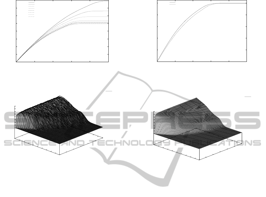
Figure 2 shows the convergence of the Monte

Carlo for day T with varying time intervals. The

maximum daily revenue seems to have converged to

around 497. Nonetheless, this convergence is slow, as

it is of order O(∆t).

The optimal rejection policy (the 2D-matrix v

k, j

−

k, j−1

), when ∆t = 1/192, can be seen in ﬁgure 3. The

ﬁgure is smoothed out using 10 iterations of 2000 runs

each. There is an increasing pattern in the spaces val-

ues, as capacity remaining goes to zero; when capac-

ity is large (Q > 60), spaces become worthless for all

times, indicating that bookings are accepted irrespec-

tive of their length of stay. Furthermore, when there

are only few spaces remaining, spaces become more

valuable with a maximum added value of around 12

monetary units. By reducing the time interval ∆t, we

managed to ‘squash in’ more customers, meaning that

we accept more bookings than before; however, such

an approach reduces the averaged added values of the

spaces.

4.2 PDE Results

Next, we present our results from the continuous-time

CONTINUOUS-TIME REVENUE MANAGEMENT IN CARPARKS

100

200

300

400

500

600

700

800

0 20 40 60 80 100

Revenue per Day

Capacity Remaining

Combined Customers

dt=1

dt=1/2

dt=1/4

dt=1/8

dt=1/24

dt=1/48

dt=1/96

dt=1/192

Figure 2: Monte-Carlo Convergence.

100

Monte-Carlo Approach

Added Value of Space

Combined Customers-Group

Capacity Remaining

Time Left

Figure 3: Monte-Carlo Optimal Rejection Policy.

PDE model and compare them with the Monte-Carlo

discrete-time model. In ﬁgure 4 we compare the ex-

pected revenues generated from the PDE model with

those from the discrete model, for day T. When ca-

pacity is adequate to meeting the demand from both

customer sets, the Monte Carlo simulations seem to

have converged to the continuous values. However,

for carparks with less than 60 spaces, Monte Carlo ap-

proach generates slightly lower revenues. A possible

explanation to this lies on the way optimal decisions

are made using the rejection algorithm. The decision

was made depending upon the total duration of stay

(added value of all periods) and not as an individual

decision at every period. If the algorithm could treat

each period independently we would expect to be able

to reject a request and reserve the space for another

potentially higher-paying customer. Nevertheless, in

our group-decision algorithm it happens that a space

might be used by a booking that comes and stays for

ten time periods because the added value of the nine

periods is too much to miss out, that we end up ﬁlling

up the tenth period too, even though that was not the

optimal decision for that period. Therefore, this prac-

tice slightly reduces the expected revenues since we

tend to slightly accept more long-stay bookings.

The question, however, is to be able to derive opti-

mal rejection policies for the case where group book-

100

200

300

400

500

0 20 40 60 80 100

Expected Revenue

Capacity Remaining

Expected Revenue when dt=1/192

Pde

MC-Group

Figure 4: Expected Revenues from PDE and Monte Carlo

computations with ∆t = 1/192.

100

Added Value of Space

Pde Approach

Combined Customers Optimized

Capacity Remaining

Time Left

Added Value of Space

Figure 5: PDE Optimal Rejection Policy.

ings are allowed.

On the one hand, calculating the correct opti-

mal rejection policy using the Monte Carlo approach

is computationally intensive as the simulations are

based on the number of paths and iterations taken; as

a result, the value surfaces produced are not smooth

enough (see ﬁgure 3) and it takes too long to be found.

If we knew the correct value surfaces, derived by

avoiding any extensive calculations, we would be able

to run the MC-Group with hundredsof thousand paths

and based on these surfaces we could make optimal

decisions and determine the optimal revenues.

On the other hand, the nature of the continuous

PDE model, generates the values quicker and the op-

timal surfaces are much smoother (see ﬁgure 5). This

is a fortunate outcome for us, but still we cannot just

replace the Monte Carlo approach with the PDE ap-

proach, since the latter does not solve the ‘full’ prob-

lem of dealing with group bookings.

Therefore, what would we aim to do now is an attempt

to generate optimal revenues using the MC-Group by

exploiting the information coming from the PDE.

4.2.1 Proposed Approach

We present the steps to be taken, as a possible ap-

proach to the problem:

ICORES 2012 - 1st International Conference on Operations Research and Enterprise Systems

(i) Solve the PDE and derive the valuesV(Q, τ) for

all states (Q,τ).

(ii) Find the optimal rejection policy by evaluating

the quantities V(Q,τ) −V(Q− 1,τ).

(iii) Choose a value for ∆t and use this policy in the

Monte Carlo to make decisions and to optimally

manage the group bookings.

(iv) Calculate the effect on the resulting revenues

and compare with the revenues obtained with-

out using the PDE policy.

(v) Based on these values, derivethe new “updated”

rejection policy.

100

200

300

400

500

600

700

800

0 20 40 60 80 100

Expected Revenue

Capacity Remaining

Expected Revenue using Pde

MC-Group

MC-Group-using pde policy

Figure 6: Effect of the PDE rejection policy on Expected

Revenues with dt = 1.

Figure 6 shows the effect on the expected revenues

when the PDE policy is used in the Monte Carlo with

the time intervals to be days (i.e. ∆t = 1). The solid

line (‘MC-Group’) shows the expected revenues us-

ing the MC-Group algorithm as in ﬁgure 2. These

values are the optimal ones when τ = 30. Thus, the

objective is to minimize the distance between the op-

timal and the approximated lines. The dashed line

(‘MC-Group-using PDE policy’) shows the expected

revenuesgenerated when the intensive simulations are

replaced by the procedure described above. The ex-

pected revenues with and without using the PDE re-

jection policy are close to each other. In particular,

we ﬁnd that their difference is always less than 8%

at all capacities. However, we believe that the pro-

posed approach will work even better for small ∆t, as

the PDE policy is derived using the continuous-time

model. Figure 7 shows the effect on the expected rev-

enues when the PDE policy is used in the Monte Carlo

with the time interval ∆t = 1/192. Clearly, the ex-

pected revenues generated are much closer and they

are always within 4% of each other.

Figure 8 shows how the rejection policies are

formed, before and after using the PDE policy. The

dashed line represents (‘MC-Group’) the optimal re-

jection policy, the solid line (‘pde’) is the PDE pol-

icy we input in the algorithm, and the dotted line

100

200

300

400

500

0 20 40 60 80 100

Expected Revenue

Capacity Remaining

Expected Revenue using Pde

MC-Group

MC-Group-using pde policy

Figure 7: Effect of the PDE rejection policy on Expected

Revenues with ∆t = 1/192.

-2

0 20 40 60 80 100

Added Value of Space

Capacity Remaining

Optimal Policy using Pde

pde

MC-Group

MC-Group-using pde policy

Figure 8: Effect of using the PDE Policy on the MC Policy

with ∆t = 1/192.

(‘MC-Group-using pde policy’) is the resulting “up-

dated” rejection policy. We observe that the proposed

approach generates a rejection policy that is signiﬁ-

cantly close to the original optimal one whilst achiev-

ing a reduction in the computation time; in particular,

the relative difference between the policies never ex-

ceed 8%.

Our results imply that even though we have used

the PDE optimal policy we could still generate near-

optimal revenues. This validates the use of the PDE

method for deriving the optimal policy and the system

could then use the Monte Carlo approach to make de-

cisions about the ‘group’ bookings.

5 CONCLUSIONS

The approach followed to solve the discrete-time

model required the use of a Monte Carlo scheme. The

rejection algorithm was developed to manage book-

ings according to the future expected revenues in the

carpark. Decisions were made optimally and the al-

gorithm has been proven to work well, as it pro-

duced greater expected revenues than all unmanaged

carparks in consideration. However, the large number

of paths and iterations used, slowed down the com-

CONTINUOUS-TIME REVENUE MANAGEMENT IN CARPARKS

putation process, and produced an optimal policy that

was not sufﬁciently smooth.

The fact that each state in the carpark can

be solved without information or dependence on

any other states, has given rise to an equivalent

continuous-time PDE approach. The model was de-

veloped, based on the probability distributions of the

bookings, inter-arrival times as well as the duration of

stay. The rejection algorithm was considered not to

solve the ‘full’ problem and, as a result, the expected

revenues were slightly different (higher) than the ob-

tained values using the Monte Carlo approach; how-

ever, a solution to the problem could be found faster

and the resulting rejection policy was much smoother.

Having this in mind, we developed an approach so

that the smooth rejection policy from the PDE could

be used in the Monte Carlo approach to solve the ‘full’

problem. Our results are promising, since we man-

aged to replicate the optimal expected revenues with

a tolerance of around 8%; a possible further improve-

ment could still be achieved.

One natural extension to the model is to con-

vert it to a dynamic pricing model where demand

intensity may be uncertain; it may be time varying

(λ = λ(t)) or, to also depend on the pricing function

(λ = λ(t, Ψ(p))) - the idea could then be extended to

multiple carparks.

REFERENCES

Arnott, R. and Rowse, J. (1999). Modeling parking. Journal

of Urban Economics, 45(1):97 – 124.

Gallego, G. and van Ryzin, G. (1994). Dynamic pricing

of inventories with stochastic demand over ﬁnite hori-

zons. Management Science, 40(8):pp. 999–1020.

Littlewood, K. (1972). Forecasting and control of passenger

bookings. 12th Sympos. Proc., pages 95–128.

Onieva, L., Mu˜nuzuri, J., Guadix, J., and Cortes, P. (2011).

An overview of revenue management in service indus-

tries: an application to car parks. The Service Indus-

tries Journal, 31(1):pp.91–105.

Teodorovi´c, D. and Luˇci´c, P. (2006). Intelligent parking

systems. European Journal of Operational Research,

175(3):1666 – 1681.

Teodorovi´c, D. and Vukadinovi´c, K. (1998). Trafﬁc con-

trol and Trasport Planning: A Fuzzy Sets and Neural

Netweorks Approach. Kluwer Academic Publishers,

Boston.

Verhoef, E., Nijkamp, P., and Rietveld, P. (1995).

The economics of regulatory parking policies: The

(im)possibilities of parking policies in trafﬁc regu-

lation. Transportation Research Part A: Policy and

Practice, 29(2):141 – 156.

Vickrey, W. S. (1969). Congestion theory and transport in-

vestment. The American Economic Review, 59(2):pp.

251–260.

Vikrey, W. S. (1994). Statement to the joint committee on

washington, dc, metropolitan problems (with a fore-

word by richard arnott and marvin kraus). Journal of

Urban Economics, 36(1):42 – 65.

Wang, L. X. and Mendel, J. (1992). Generating fuzzy rules

by learning from examples. Systems, Man and Cyber-

netics, IEEE Transactions on, 22(6):1414 –1427.

Young, W., Thompson, R. G., and Taylor, M. A. (1991). A

review of urban car parking models. Transport Re-

views, 11(1):63–84.

Zhao, Y., Triantis, K., Teodorovic, D., and Edara, P. (2010).

A travel demand management strategy: The down-

town space reservation system. European Journal of

Operational Research, 205(3):584 – 594.

ICORES 2012 - 1st International Conference on Operations Research and Enterprise Systems