VEHICLE CLASSIFICATION USING EVOLUTIONARY FORESTS

Murray Evans, Jonathan N. Boyle and James Ferryman

Computational Vision Group, School of Systems Engineering, University of Reading, Reading RG6 6AY, U.K.

Keywords:

Vehicle classiﬁcation, Evolutionary forests.

Abstract:

Forests of decision trees are a popular tool for classiﬁcation applications. This paper presents an approach to

evolving the forest classiﬁer, reducing the time spent designing the optimal tree depth and forest size. This

is applied to the task of vehicle classiﬁcation for purposes of veriﬁcation against databases at security check-

points, or accumulation of road usage statistics. The evolutionary approach to building the forest classiﬁer is

shown to out-perform a more typically grown forest and a baseline neural-network classiﬁer for the vehicle

classiﬁcation task.

1 INTRODUCTION

Vehicle classiﬁcation is a potentially very useful tool.

In the context of border security checkpoints, auto-

matic classiﬁcation of vehicles could be used in con-

junction with automatic number-plate recognition to

provide veriﬁcation that the type of car registered

against the plate number matches the car observed at

the checkpoint. Mismatches can indicate stolen or un-

licenced vehicles which should be more thoroughly

checked. Alternatively, a camera observing a road

or gate could be used to determine statistics of ve-

hicle types that pass through, providing information

that can be of use in future road planning activities.

At a border checkpoint, passenger vehicles

(busses, cars) and light goods vehicles (vans) are often

split from heavy goods vehicles. This paper presents

the results of research developing a classiﬁer capa-

ble of distinguishing between different sub-classes of

passenger vehicles: hatchbacks, saloons, estate cars,

sports-utility vehicles, sports-cars etc. At this level,

the information provided can be useful for veriﬁca-

tion against the registered details of a vehicle. For

instance, vehicle registration information will often

store details of the make and model of a car against

its registration details. In the UK, a Ford Focus can

be either an estate or a hatchback, so an SUV trav-

elling with registration plates beﬁtting a Ford Focus

could indicate foul play, and should arouse suspicion.

Although previously published works have consid-

ered multiple vehicle classes, few have considered the

task of vehicle classiﬁcation beyond the car/bus/truck

level.

To achieve the classiﬁcation, it was decided to ex-

plore the potential of forest classiﬁers. Forests are

ensembles of decision trees, and have seen much in-

terest in the vision community after the publication

of (Lepetit and Fua, 2006). Of particular interest have

been the so called randomised forests. Forest classi-

ﬁers are appealing in part because of their simplicity,

but equally from their fast run-time performance, in-

herent ability to deal with multiple classes, and the

simplicity with which wildly different primitive clas-

siﬁers can form the building blocks of the forest.

This paper proposes constructing the forest clas-

siﬁer using an evolutionary approach, resulting in a

classiﬁer that is generally smaller and of superior per-

formance to a forest grown in the original manner.

The remainder of this paper is structured as fol-

lows: Section 2 will discuss previous works on vehi-

cle classiﬁcation. Section 3 will then detail the data

set created for the experiments. The developed classi-

ﬁer will be introduced in Section 4 and then evaluated

in Section 5, before Section 6 concludes and consid-

ers future work.

2 RELATED WORK

Previous research into the area of vehicle classiﬁca-

tion has shown some success. Classiﬁcation is per-

formed in (Gupte et al., 2002) to split vehicles in a

highway scene into Truck and non-truck classes by

estimating the size of the vehicle using calibration in-

formation, an approach similarly taken by (Shi et al.,

2007). The calibration requirement is avoided in (Av-

387

Evans M., N. Boyle J. and Ferryman J. (2012).

VEHICLE CLASSIFICATION USING EVOLUTIONARY FORESTS.

In Proceedings of the 1st International Conference on Pattern Recognition Applications and Methods, pages 387-393

DOI: 10.5220/0003763603870393

 SciTePress

ery et al., 2004) by determining the length of motion

blobs and determining the statistics for the current

view to split into long and short vehicles. The cal-

ibration step is also avoided by (Hsieh et al., 2006),

which automatically determines the lanes of the road

and normalises the size of the detected vehicles by

the width of the lane at the part of the image. Vehi-

cles are classiﬁed based on their size and a feature

termed “linearity” into cars, mini-vans, trucks and

“van-trucks”. (Huang and Liao, 2004) also make use

of vehicle size from a side proﬁle view of a highway,

but also incorporate further measurements of the as-

pect ratio and compact ratio of the motion silhouettes

to get a ﬁner grained classiﬁcation considering seven

classes.

Earlier work using a model ﬁtting approach can

be seen in (Sullivan et al., 1996) which showed

promising results classifying cars versus vans, again

in a highway scenario. A related approach was

later taken by (Buch et al., 2008) using the possi-

ble classiﬁcations: Bus/Lorry, Van, Car/Taxi, Motor-

bike/bicycle. The advantage of such model based ap-

proaches should be a reduction in view-point depen-

dence, though building the models could be expensive

and prone to error.

Other approaches include the use of Gabor ﬁlters

and a minimum-distance classiﬁer (Ji et al., 2007),

using normalised side-proﬁle images of the vehicles.

(Zhang et al., 2006) perform the classiﬁcation using

“Eigen-vehicles” (a reference to Eigenfaces), along

with PCA and a support vector machine. (Zhang

et al., 2008) use a transformation-ring-projection with

wavelet fractal signatures to describe side-proﬁle ve-

hicle segmentations for classiﬁcation. Classiﬁcation

and tracking are considered together in (Morris and

Trivedi, 2006), and (Negri et al., 2006) use frontal

views to go as far as classifying individual models of

cars.

3 DATA PREPARATION

In common UK parlance, cars can be grouped into

one of the following types: hatchbacks, saloons, es-

tates, off-roaders or Sports Utility Vehicles (SUVs),

sports-cars, convertibles and people-carriers. Add to

this, there are vans, busses, trucks, pickups and lor-

ries. To collect a suitable data-set, a camera was

erected at one of the main entrance/exit gates at the

University of Reading, looking perpendicular across

the entrance road. This recorded the morning rush-

hour, accumulating a total of approximately four

hours of footage. The orientation of the camera was

chosen to capture as close to a side-proﬁle of the pass-

ing cars as was possible, as the side-proﬁle was con-

sidered to be the most discriminating between the dif-

ferent classes of vehicles.

A motion detector (Zivkovic, 2004) was used to

detect frames in the video where the quantity of mo-

tion in a pre-deﬁned section towards the centre of

the image passed a threshold, indicating the presence

of a vehicle. A wheel detector was used to deter-

mine the location of the wheels of the vehicle, and

then scaling and cropping was applied to both the

RGB and motion-mask images, such that the wheels

occupied a pre-deﬁned location in the resulting nor-

malised images. The normalised images were sized at

200 ×85 pixels, with the front and back wheels cen-

tred at (50, 80) and (150, 80) respectively. The result-

ing images were then manually parsed to determine

their correct classiﬁcation, and to verify robust nor-

malisation.

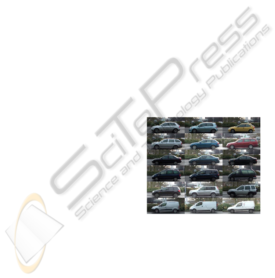
Examples of the normalised images for several of

the observed vehicle classes are shown in Figure 1,

along with example motions masks in Figure 2. The

resulting image database contained example images

in the classes and quantities listed in Table 1. It is

quite clear that a strong bias exists for vehicles ﬁtting

into the hatchback category.

Figure 1: Examples of the normalised vehicle images. From

top to bottom the images depict samples from the classes:

hatchback, estate, saloon, people-carrier, SUV and van.

4 FOREST CLASSIFIER

To classify the vehicle images, an “evolutionary for-

est” classiﬁer has been developed. This fuses the

traditional forest classiﬁer (an ensemble of decision

trees) (Breiman, 2001), with techniques from genetic

algorithms to evolve a forest optimised for the classi-

ﬁcation task.

ICPRAM 2012 - International Conference on Pattern Recognition Applications and Methods

388

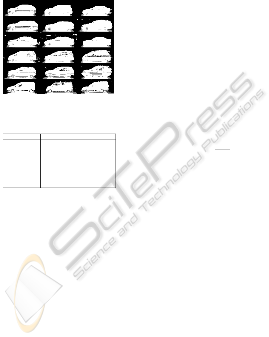
Figure 2: Examples of the normalised mask images accom-

panying the normalised RGB images depicted in Figure 1.

Table 1: Classes and number of example images acquired,

as well as example training/testing splits.

class id total training testing

hatchback 1 7027 351 6676

estate 2 1163 58 1105

saloon 3 1640 82 1558

convertible 4 342 50 292

sports-car 5 173 50 123

people-carrier 6 680 50 630

SUV 7 543 50 493

van 8 1246 62 1184

Recently, randomised decision forests have been

of great interest. These grow a set of decision trees

where each decision node of the tree is conﬁgured

to exploit a randomly chosen classiﬁer from a set of

available classiﬁers, often with randomly initialised

parameters that are optimised to produce the best split

of the training examples. Typically, only binary deci-

sion trees are used, where each node has two children.

These randomised decision forests can be effective in

many scenarios, perhaps most famously in the Mi-

crosoft Kinect player tracking system (Shotton et al.,

2011), however it can be unclear as to how large the

forest should be, and how deep each tree should be

permitted to become. Furthermore, while each tree is

optimised to be the best classiﬁer it can be, the trees

are not optimised to work together to produce the best

forest that can be produced.

This work considers an evolutionary approach to

growing the forest ensuring that every tree that is a

part of the forest is there to optimise the forest’s over-

all performance.

4.1 Decision Tree Nodes

Each decision tree in the forest is a binary tree where

each node is a primitive binary classiﬁer. Given an

input, each node can either send the input to its left

or right child. For the purposes of the vehicle classi-

ﬁcation task four very simple low-level image based

classiﬁers have been implemented.

4.1.1 Pixel Difference Node

This ﬁrst node has ﬁve parameters, namely the (x, y)

image coordinates of two pixels in the image, and a

threshold value t

. The colour p

and p

of each pixel

is extracted and represented in CIELAB space, then

the Euclidean difference is computed between the two

colours, and compared to a threshold. If the result is

larger than the threshold, the second child is activated,

otherwise, the ﬁrst child is activated. If c represents

the child, then the node’s function can be represented

by the equation:

c =



1 if t

√

·p

0 otherwise

(1)

4.1.2 Edge Orientation Node

The input image I can be transformed to the two chan-

nel image E representing the magnitude and orienta-

tion of gradients in the image. A decision node can

be created that checks if, for a given pixel (x, y), the

magnitude is above a threshold t

and the orientation

is between the values t

→t

. This node therefore

has ﬁve parameters (the pixel co-ordinates and three

thresholds). Let m and o be the gradient magnitude

and orientation at (x, y), then the appropriate child is

selected from:

c =



1 if (m > t

) ∧(t

< o < t

)

0 otherwise

(2)

4.1.3 Chamfer Node

The edge magnitude image can be thresholded to pro-

duce a binary edge image. This in turn can be used to

produce a distance transform image, or chamfer im-

age C where every pixel is valued by its distance from

the nearest edgel. A very simple node can then be

created that, given two pixels as input, selects the ap-

propriate child based on whether the ﬁrst or second

pixel has a larger value in C.

c =



1 if C(x

, y

) > C(x

, y

)

0 otherwise

(3)

VEHICLE CLASSIFICATION USING EVOLUTIONARY FORESTS

389

4.1.4 Mask Node

The ﬁnal node takes in the binary motion mask M that

was created at the same time as the RGB image I. For

a given pixel, this node selects a child based only on

whether the pixel is active in the mask image, or not.

c =



1 if M(x, y) > 0

0 otherwise

(4)

4.2 The Evolutionary Forest

To create a randomised forest, each tree is grown one

by one. First, a classiﬁer is selected at random for

the root node, and the parameters which create the

optimal split of the input data determined (see sec-

tion 4.2.2). The split data are then sent to the child

nodes, and so on, until a maximum tree depth is

achieved, or a split of the data contains only one class

type.

When an unseen testing example is presented to

the forest, it will pass through each tree and reach a

leaf node, providing information on what the likely

class of the unknown image is. For instance, if the

leaf node recorded 200 instances of a hatchback, and

only one instance of SUV, the probability would be

that the unknown image also represents a hatchback.

The vector of class counts for all leaf nodes can be

accumulated to determine a belief as to the most ap-

propriate class for the input image.

In this approach, each tree is an independently op-

timised classiﬁer, and the forest result a majority be-

lief. There exists some prior work in using evolution-

ary approaches to create decision trees (Papagelis and

Kalles, 2001), however in this work the aim is not to

produce a population of independently optimal deci-

sion trees, but rather to evolve a set of trees that work

together in an optimal forest.

4.2.1 Constructing the Evolutionary Forest

To begin creating the forest, the ﬁrst decision tree

must be created. An initial set of short decision trees

is grown. This will form the population from which

the ﬁrst tree of the ﬁnal forest classiﬁer is evolved.

Each of the initial trees is grown using a subset of the

whole set of training images T . The trees are then

evaluated against their ability to classify the whole of

T . The worst w% of trees are then exposed to replace-

ment by one of the following genetic operators:

1. Cross-over: The poor performing tree t

is re-

moved from the set of trees, and replaced by a

new tree that is the product of a cross-over “breed-

ing” of two trees with better performance. This

involves selecting a random node on each of the

better trees, and swapping them, children and all.

This results in two trees, the shorter of which is

selected as the replacement tree.

2. Regeneration: The poor performing tree t

is re-

moved from the set of trees and replaced by a

completely new tree.

3. Mutation: A node is selected in the poorly per-

forming tree t

. The node is replaced by a differ-

ent node with randomly selected parameters.

After a number of iterations (this can be a ﬁxed

number, or a number based on the current best per-

formance of the population), the genetic process is

stopped. The best performing tree is taken from the

set of trees, and becomes the ﬁrst tree of the ﬁnal for-

est classiﬁer.

Now, the process repeats, adding trees one at a

time to the ﬁnal forest, However, after the ﬁrst op-

timisation, the deﬁnition of the “best” tree is slightly

altered. No longer is it desirable to produce an opti-

mal, stand-alone decision tree. Rather, what is sought

is the tree that best augments the current ﬁnal forest.

The evaluation criteria and the algorithm to optimise

the individual trees will now be discussed in the re-

maining parts of this section. The training algorithm

is summarised in Figure 3.

Let T be the set of training images

Create an empty forest F

while no. of trees < maximum:

Create V , a random subset of T

Create a set of decision trees, F

for c = 0 to max no. iterations:

Train the trees in F

Evaluate the trees in F

Replace the worst w% of trees in F

Add the best tree in F

to F

Perform a ﬁnal training of F

Figure 3: Pseudocode of evolutionary forest algorithm.

4.2.2 Optimising Tree Nodes

When growing the initial trees, it is useful to opti-

mise the parameters of a node to produce the “best”

possible split of the data. This is achieved by using

a greedy search of the parameters to maximise the in-

formation gain between the input data to the node, and

the two output sub-sets, identical to the approach used

in (Shotton et al., 2011).

ICPRAM 2012 - International Conference on Pattern Recognition Applications and Methods

390

4.2.3 Evaluating Tree Performance

On the initial iteration that produces the ﬁrst tree for

the ﬁnal forest, the evaluation function for the trees

is set such that the evolutionary process is attempt-

ing to produce the best possible stand-alone decision

tree. This performance is captured by the following

equation:

φ( f

) = 0.3¯z + 0.7 min

Z(i, j) (5)

Here, Z(i, j) is the number of images that the tree

correctly classiﬁed of class h

, normalised by the

number of examples of class h

that were shown to

the tree. Meanwhile, ¯z is used to indicate the median

of Z(i, j) over the possible classes h

. This equation

is structured to favour a tree that performs reasonably

well across all of the possible classes, rather than a

tree that excels at any one class but is wholly wrong

on some others, and the parameters 0.3 and 0.7 bal-

ance the equation to encourage a jack-of-all trades

classiﬁer which has generally provided the best start-

ing point for the evolutionary process.

Once the ﬁrst tree has been selected, the optimi-

sation function used to design subsequent trees alters.

Rather than trying to make a tree that is an optimal

classiﬁer of the data, the aim is to produce a tree that

best augments the existing forest. This is a more sub-

tle equation to produce.

Let F

be the ﬁnal forest that the algorithm is try-

ing to produce, and F

be the population of trees that

are being optimised to produce the i’th tree for F

(meaning that F

contains i −1 trees).

For any given image I with known class h, F

can

be used to produce a classiﬁcation h

. In doing so, it

will also produce the belief vector h

, which is the ac-

cumulated beliefs of all the i −1 leaf nodes reached

during the classiﬁcation process. In an ideal classi-

ﬁer, all but the belief in the correct class will be 0.

More realistically, the desire will be that the belief in

the correct class is larger than the belief in each of

the other classes. The larger this difference, the more

conﬁdent the classiﬁcation.

As such, for a given image, it is possible to calcu-

late h

as the belief of the forest F

, as well as h

the belief of the forest F

, which is the forest F

aug-

mented by a tree in F

. The effectiveness of the tree

to improve or complement the performance of F

can

then be written as:

σ( f

∈ F

) =

∑



−m

)) −(c

−m

))



(6)

where c

and c

are the values of h

and h

for the

correct classiﬁcation of the image I, while m

and m

the largest values in h

and h

. If the forest is correct,

the term c −m will be positive, and the more conﬁ-

dent the classiﬁcation, the larger the positive value. If

the augmented forest performs better then σ( f

) will

be positive, and the better it performs, the more pos-

itive it becomes. In this way, F

is breeding trees de-

signed to improve the performance of the ﬁnal forest

, rather than trees that operate as expert independent

classiﬁers.

5 RESULTS

To evaluate the performance of the classiﬁer, the im-

age dataset was randomly split such that for each

class h

with n

training examples there were at least

max(50, 0.05 ×n

) images removed from the training

set to the testing set. Table 1 shows an example split

of the data, and also gives each class an identifying

number corresponding to the numbers in the confu-

sion matrices in Table 2.

The classiﬁcation performance of the genetically

optimised classiﬁer is compared to a traditionally

grown randomised forest, as well as “baseline” results

from a multi-layer perceptron neural network. The

classiﬁcation results of each classiﬁer are displayed

as confusion matrices. Given the set of images for a

speciﬁc class (e.g. hatchback, row 1), the columns

specify the percentage of images classiﬁed, or mis-

classiﬁed, as each of the possible classiﬁcations. A

perfect classiﬁer will produce 100% along the diago-

nal, and 0% everywhere else. The confusion matrices

in Table 2 show average values over twenty different

training/testing splits.

The genetic forests typically reach maximum per-

formance against the testing set by about 30 to 45

trees, as such, all were grown to a size of 50 trees. In-

dividual trees in the forests reached a maximum depth

of 16 levels, however, the median depth for any one

tree is only 4.

The randomised forests were each grown to a

maximum depth of 11 nodes, with again 50 trees per

forest, a size empirically suggested as near-optimal

for the classiﬁcation task in hand. Note that this is a

far larger forest (due to the increased depth) than the

evolved forest.

For comparison with other traditional classiﬁca-

tion approaches, a multi-layer perceptron was also

trained on the data, using gradient images as the in-

put. The results of this approach are the weakest of

the tested methods, showing that the forest, and evo-

lutionary forest, are an excellent choice for this clas-

siﬁcation task.

VEHICLE CLASSIFICATION USING EVOLUTIONARY FORESTS

391

Table 2: Classiﬁcation results for (from top to bottom), the

evolutionary forest, randomised forest, and neural network.

0 1 2 3 4 5 6 7

1 97.2 0.4 0.6 0.0 0.5 0.8 0.1 0.4

2 5.1 81.6 7.2 0.6 0.4 4.1 0.6 0.4

3 0.5 2.7 90.1 2.5 4.1 0.0 0.0 0.1

4 8.7 1.1 10.7 76.2 3.2 0.0 0.2 0.0

5 2.7 0.0 6.6 1.3 89.3 0.0 0.0 0.0

6 13.5 3.7 0.0 0.0 0.0 75.7 6.6 0.5

7 4.2 2.5 0.1 0.6 0.0 5.5 85.3 1.8

8 2.5 0.7 0.0 0.0 0.0 2.6 1.9 92.4

0 1 2 3 4 5 6 7

1 95.6 0.4 0.2 0.1 0.8 2.8 0.0 0.1

2 6.5 63.8 12.3 1.6 0.8 13.2 1.8 0.1

3 0.9 3.1 86.9 5.0 3.8 0.1 0.1 0.0

4 15.8 0.6 18.1 63.2 2.2 0.1 0.1 0.0

5 6.7 0.0 15.0 2.9 75.5 0.0 0.0 0.0

6 18.3 0.9 0.0 0.0 0.0 71.0 9.7 0.0

7 6.9 1.4 0.1 0.8 0.0 18.5 71.9 0.4

8 5.0 0.6 0.0 0.0 0.0 9.0 4.6 80.6

0 1 2 3 4 5 6 7

1 92.9 1.6 2.1 0.2 2.3 0.4 0.4 0.1

2 18.3 58.5 6.4 11.1 1.0 3.8 0.3 0.8

3 10.3 2.2 77.0 6.9 1.2 0.3 1.8 0.4

4 11.4 3.1 20.6 56.7 2.7 0.5 2.5 2.4

5 16.1 0.2 4.2 0.1 72.7 1.2 4.6 0.9

6 10.0 13.4 0.7 1.2 9.8 54.9 3.0 7.0

7 3.5 1.0 5.3 2.5 4.4 2.5 69.9 11.0

8 0.8 1.7 0.9 3.9 2.0 5.3 6.5 79.0

6 CONCLUSIONS AND FUTURE

WORK

This paper has considered the application of forest

classiﬁers to the task of vehicle classiﬁcation, propos-

ing in the process a method of growing the forest by

use of an evolutionary approach. Compared to the

typical randomised forest, the genetic forest showed

superior performance, and also performed better than

a baseline neural network.

Future work will aim to extend the current imple-

mentation to classify vehicles into make and model

categories, alternative image features to exploit at

each low-level classiﬁer node, as well as determin-

ing the efﬁcacy of the evolutionary forest approach in

other contexts.

ACKNOWLEDGEMENTS

This work was partially funded by the EU FP7 project

EFFISEC with grant No. 217991.

However, this paper does not necessarily represent the

opinion of the European Community, and the European

REFERENCES

Avery, R., Wang, Y., and Scott Rutherford, G. (2004).

Length-based vehicle classiﬁcation using images from

uncalibrated video cameras. In Intelligent Transporta-

tion Systems, 2004. Proceedings. The 7th Interna-

tional IEEE Conference on, pages 737 – 742.

Breiman, L. (2001). Random forests. Machine Learning,

45:5–32. 10.1023/A:1010933404324.

Buch, N., Orwell, J., and Velastin, S. (2008). Detection and

classiﬁcation of vehicles for urban trafﬁc scenes. In

Visual Information Engineering, 2008. VIE 2008. 5th

International Conference on, pages 182 –187.

Gupte, S., Masoud, O., Martin, R., and Papanikolopoulos,

N. (2002). Detection and classiﬁcation of vehicles. In-

telligent Transportation Systems, IEEE Transactions

on, 3(1):37 –47.

Hsieh, J.-W., Yu, S.-H., Chen, Y.-S., and Hu, W.-F.

(2006). Automatic trafﬁc surveillance system for vehi-

cle tracking and classiﬁcation. Intelligent Transporta-

tion Systems, IEEE Transactions on, pages 175 – 187.

Huang, C.-L. and Liao, W.-C. (2004). A vision-based ve-

hicle identiﬁcation system. In Pattern Recognition,

2004. ICPR 2004. Proceedings of the 17th Interna-

tional Conference on, volume 4, pages 364 – 367

Vol.4.

Ji, P., Jin, L., and Li, X. (2007). Vision-based vehicle

type classiﬁcation using partial gabor ﬁlter bank. In

Automation and Logistics, 2007 IEEE International

Conference on, pages 1037 –1040.

Lepetit, V. and Fua, P. (2006). Keypoint recognition using

randomized trees. Transactions on Pattern Analysis

and Machine Intelligence, 28(9):1465–1479.

Morris, B. and Trivedi, M. (2006). Improved vehicle clas-

siﬁcation in long trafﬁc video by cooperating tracker

and classiﬁer modules. In IEEE International Con-

ference on Advanced Video and Signal based Surveil-

lance.

Negri, P., Clady, X., Milgram, M., and Poulenard, R.

(2006). An oriented-contour point based voting algo-

rithm for vehicle type classiﬁcation. In Pattern Recog-

nition, 2006. ICPR 2006. 18th International Confer-

ence on, pages 574 –577.

Papagelis, A. and Kalles, D. (2001). Breeding decision trees

using genetic algorithms. In International Conference

on Machine Learning, Proceedings of.

Shi, S., Qin, Z., and Xu, J. (2007). Robust algo-

rithm of vehicle classiﬁcation. In Software Engineer-

ing, Artiﬁcial Intelligence, Networking, and Paral-

lel/Distributed Computing, 2007. SNPD 2007. Eighth

ACIS International Conference on, pages 269 –272.

Shotton, J., Fitzgibbon, A., Cook, M., Sharp, T., Finocchio,

M., Moore, R., Kipman, A., and Blake, A. (2011).

Real-time human pose recognition in parts from a sin-

gle depth image. In Computer Vision and Pattern

Recognition, IEEE Conference on.

Community is not responsible for any use which may be

made of its contents.

ICPRAM 2012 - International Conference on Pattern Recognition Applications and Methods

392

Sullivan, G. D., Baker, K. D., Worrall, A. D., Attwood,

C. I., and Remagnino, P. R. (1996). Model-based ve-

hicle detection and classiﬁcation using orthographic

approximations. In 7th British Machine Vision Con-

ference.

Zhang, C., Chen, X., and bang Chen, W. (2006). A pca-

based vehicle classiﬁcation framework. In Data En-

gineering Workshops, 2006. Proceedings. 22nd Inter-

national Conference on, page 17.

Zhang, D., Qu, S., and Liu, Z. (2008). Robust classiﬁca-

tion of vehicle based on fusion of tsrp and wavelet

fractal signature. In Networking, Sensing and Con-

trol, 2008. ICNSC 2008. IEEE International Confer-

ence on, pages 1788 –1793.

Zivkovic, Z. (2004). Improved adaptive gaussian mixture

model for background subtraction. In Pattern Recog-

nition, 2004. 17th International Conference on, pages

28–31.

VEHICLE CLASSIFICATION USING EVOLUTIONARY FORESTS

393